Escuela Técnica Superior de
Ingenieros de Caminos, Canales y Puertos
Experimental and computational
micromechanical study of
fiber-reinforced polymers
Tesis doctoral
Luis Pablo Canal Casado
Licenciado en Ciencias Físicas
Ingeniero de Materiales
Caminos, Canales y Puertos
Universidad Politécnica de Madrid
Experimental and computational
micromechanical study of
fiber-reinforced polymers
Tesis doctoral
Luis Pablo Canal Casado
Licenciado en Ciencias Físicas
Ingeniero de Materiales
Directores de la tesis
Carlos González Martínez
Dr. Ingeniero de Caminos, Canales y Puertos
Profesor Titular de Universidad
Javier Segurado Escudero
Dr. Ingeniero de Materiales
Profesor Titular de Universidad
Agradecimientos III
Resumen VI
Abstract IX
1 Introduction 1
1.1 Background . . . 1
1.2 Damage mechanisms in FRPs . . . 5
1.3 Failure criteria in FRPs . . . 8
1.4 Micromechanical models of composite materials . . . 11
1.5 Analytical micromechanics . . . 12
1.5.1 Mean field approaches . . . 12
1.5.2 Variational bounding methods . . . 14
1.6 Computational micromechanics . . . 14
1.6.1 Periodic microfield approaches . . . 14
1.6.2 Embedded cells . . . 21
1.7 Constitutive models for FRPs microconstituents . . . 23
1.7.1 Plastic behavior of the matrix . . . 24
1.7.2 Matrix damage behavior . . . 29
1.7.3 Damage-plasticity coupled model of the matrix . . . 39
1.7.4 Fiber-matrix interface . . . 42
2 Characterization of the transverse properties of unidirectional FRPs 45
2.1 Material . . . 45
2.2 Compressive properties determination . . . 46
2.2.1 Experimental results . . . 47
2.3 Tensile properties determination . . . 52
2.3.1 Experimental results . . . 53
2.4 Concluding remarks . . . 53
3 Micromechanical characterization of FRPs constituents 57 3.1 Matrix characterization . . . 57
3.1.1 Determination of the Young’s modulus and compressive yield stress . . . 58
3.2 Fiber-matrix interface characterization . . . 65
3.2.1 Interface strength determination . . . 65
3.2.2 Interface toughness . . . 73
3.3 Concluding remarks . . . 73
4 Fracture behavior of FRPs 75 4.1 Experimental techniques . . . 77
4.2 Experimental results . . . 79
4.2.1 Fracture mechanisms . . . 81
4.3 Computational model . . . 84
4.3.1 Simulation of the transverse tension test . . . 84
4.3.2 Simulation of the three-point bending test . . . 91
4.4 Concluding Remarks . . . 100
5 In situ SEM compression test 105 5.1 Experimental techniques . . . 106
5.2 DIC in heterogeneous materials . . . 108
5.3 Experimental Results . . . 116
5.3.1 Elastic loading . . . 118
5.4 Numerical model . . . 127
5.4.1 Elastic deformation . . . 130
5.4.2 Inelastic deformation . . . 133
5.5 Concluding Remarks . . . 137
6 Computational prediction of the failure locus 139 6.1 Introduction . . . 139
6.2 Computational model . . . 140
6.3 Results . . . 143
6.4 Concluding Remarks . . . 152
7 Conclusions and future work 155 7.1 Conclusions . . . 155
7.2 Future work . . . 156
7.2.1 Experimental work . . . 157
En primer lugar, quiero expresar mi sincero agradecimiento a mis directores de tesis, Javier Segurado y Carlos González, por las numerosas enseñanzas transmitidas durante el transcurso de esta tesis. A pesar de que a lo largo de este periodo sus obligaciones profesionales y personales se han visto sensiblemente incrementadas, siempre han sabido demostrar una plena dedicación, disponibilidad y proximidad.
Deseo agradecer a Javier LLorca la oportunidad de trabajar en el grupo de ma-teriales compuestos, la orientación científica y su inestimable ayuda en la realización de este trabajo.
Este agradecimento debo extenderlo a todos y cada uno de los miembros del Departamento de Ciencia de Materiales, por su amabilidad y su ayuda en incontables ocasiones. Deseo mencionar y agradecer todos los buenos momentos compartidos con mis compañeros y amigos Joaquín, José Miguel, Bea, Borja, Álex, Els, Mónica, Fran, Gustavo, Elena y a muchos otros que he podido olvidar en esta lista, pero que también merecen estar. En especial, agradezco a David, Álvaro y Konstantina por su gran amistad, apoyo, consejo y mucha ayuda durante la realización de esta tesis.
Agradezco a Jon Molina, del Instituto IMDEA-Materiales, su gran colaboración para la realizar los ensayos in situ. En la misma institución quiero mencionar a Marcos y a Sergio por su ayuda con el nanoindentador y las simulaciones, pero sobre todo por su compañerismo y gran amistad.
Quiero mencionar también a todos los amigos fuera del ámbito laboral, por todo lo que hemos compartido durante estos años.
Los materiales compuestos de matriz polimérica reforzados por fibras tienen pro-piedades mecánicas muy adecuadas para su utilización en aplicaciones estructurales. Estos materiales, debido a los altos valores de rigidez y resistencia específica, están desplazando a materiales convencionales en numerosas aplicaciones en las que se re-quiere la mejor relación entre las prestaciones mecánicas y el peso. Hoy en día, en el diseño de estructuras con materiales compuestos se utilizan criterios de fallo con base fenomenológica que requieren de un gran número de ensayos experimentales para obtener todos los parámetros del material necesarios y garantizar la seguridad de los componentes construidos. Este inconveniente en la aplicación de materiales compuestos se debe a la complejidad de su comportamiento mecánico, que está go-bernado por diversos procesos que ocurren a nivel microscópico. Este es el caso, por ejemplo, de procesos como la concentración de tensiones y deformaciones, las deco-hesiones entre las distintas fases del compuesto o el fallo de los microconstituyentes, que determinan las propiedades finales del material.
com-puesto sometido a cargas en la dirección perpendicular al refuerzo comenzaba en las intercaras fibra/matriz y se propagaba a través de la unión de las intercaras dañadas mediante la rotura de los ligamentos de matriz entre fibras decohesionadas.
El comportamiento mecánico del laminado hasta rotura se modeló mediante la simulación por elementos finitos de modelos micromecánicos que representaban la microestructura real del material. Siguiendo las observaciones experimentales, el modelo numérico incluía la decohesión de las intercaras y la rotura de la matriz. Los resultados de las simulaciones mostraron un buen acuerdo con los experimentos tanto en su respuesta macroscópica como en los mecanismos de deformación y daño microscópicos.
Fiber-reinforced polymers (FRPs) exhibit outstanding mechanical properties, ideal for their use in structural applications. Due to the high specific values of stiffness and strength, these composites are replacing conventional materials in applications where a superior mechanical performance in combination with weight saving is necessary. However, the lack of reliable and experimentally contrasted models to accurately predict the failure strength of FRPs makes the optimization process of composite structures to be carried out by means of a costly and time-consuming trial-and-error approach, which requires an immense burden of testing and restricts the promising improvements of the use of composites. This difficulty in the simulation of mechan-ical behavior and damage of composites is due to the fact that an accurate model should account for the phenomena which take place at the micron scale, which is in the size of the reinforcement. This is the case, for instance, of the stress and strain concentration, decohesion of the reinforcement and damage of the material constituents.
and continues with the subsequent propagation of the damage by the link up of the interface fractures by breaking the matrix ligaments between debonded fibers.
The mechanical behavior of the unidirectional laminate until final fracture was modeled by the finite element simulation of micromechanical models which repre-sented the microstructure of the real material. Following the previous experimental observation, the interface decohesion and the failure of the matrix were included in the computational model. The simulation results were in very good agreement with the experiments in terms of the macroscopic response and of the microscopic mechanisms.
Introduction
1.1
Background
Composite materials are created by the combination of two or more different constituents or phases which remain separate and distinct within the composite mi-crostructure. The combination of the different mechanical properties of each indivi-dual constituent brings the opportunity to tailor a specific material with the required properties for a given application. For this reason, composite materials are playing nowadays an increasing role in technological industries such as aerospace, automobile, construction, energy or biomedical. It is possible to find good examples of technolog-ical applications with ceramic matrix and metal matrix composites in cutting tools, armors for military vehicles, disc brakes for sport cars or gas turbine components. However, among all the high performance composite materials, fiber-reinforced poly-mers (FRPs) are the most extensively used for lightweight structural applications.
load-bearing phase, while the matrix is mainly used to maintain the fibers oriented in the design direction. Due to their outstanding specific mechanical properties and the ma-ture level of the processing and quality control techniques, FRPs are extensively used nowadays in structural applications where weight saving is a mandatory requirement. Good examples of the FRPs applications can be found in the aerospace industry: the A380, the last civil Airbus aircraft, contains up to 25% in weight of composite materi-als (used for wings, fuselage sections and tail surfaces) or the Boeing 787 Dreamliner which claims to be the first airliner with a fully composite fuselage manufactured with advanced carbon components technologies. Nowadays, engineers have excellent tools for predicting the load distribution throughout the structure when the material behavior is linear-elastic, but predictions become problematic once damage begins. The fundamental difficulty is that damage in these engineering materials involves extremely complicated nonlinear processes acting at different scales, from the atomic to the structure level.
The standard strategy to tackle the failure predictions in FRPs starts from a numerical analysis of the whole structure in a top-bottom approach. This initial
evaluation identifies hot spots in which damage is likely to occur, and these regions are subjected to further refined analysis. Nonlinear constitutive models based on phenomenological approaches are used to predict the material behavior until frac-ture. Although this strategy focuses on engineering necessities, it has also important limitations. An extensive experience and costly testing campaigns are necessary to calibrate these models employed in the critical regions. Innovations in materials are limited because of the lack of reliable data to assess the onset and propagation of damage upon loading. And finally, the extrapolation of current knowledge to different loading/environmental conditions is problematic due to the phenomenological nature of the models.
Recent developments in multiscale simulations, together with increased computa-tional power and improvements in modeling tools, are enabling an alternative strategy that overcomes the limitations of thetop-bottom approach. Nowadays, it is beginning
new hierarchical,bottom-up approach is being developed to carry out virtual tests of
composite materials and structures (LLorca and González, 2011). The overall mul-tiscale simulation scheme is depicted in Fig.1.1 and takes advantage from the fact that composite structures are made up of laminates which in turn are obtained by stacking individual plies with different fiber orientation. This leads to three different entities (ply, laminate and component) whose mechanical behavior is characterized by three different length scales, namely fiber diameter, ply and laminate thickness, respectively. Fiber diameters are of the order of 5-20µm, while ply thicknesses are in
the range 100-300µm and standard laminates are several mm in thickness and above.
This clear separation of length scales is very useful to carry out multiscale model-ing by computmodel-ing the properties of one entity (e.g. individual plies) at the relevant length scale, homogenizing the results into a constitutive model, and passing this information to the simulations at the next length scale to determine the mechanical behavior of the larger entity (e.g. laminate). Thus, multiscale modeling is carried out through the transfer of information between different length scales rather than by coupling different simulation techniques.
These results are finally used within the framework of computational mechanics to obtain the response until fracture of structural components made of composites.
1.2
Damage mechanisms in FRPs
1
2 3
(a) (b)
(e) (d)
(c)
Figure 1.3: X-ray computed tomography showing different failure micromecha-nisms in a [90/−45/45/0/45/−45/90] composite laminate loaded in tension parallel to the plies with fibers oriented at 0◦. Fiber fracture is dominant in the 0◦ plies, while matrix cracking parallel to the fibers dictates the failure of the 90◦ and 45◦ plies. In addition, matrix cracks led to interface delamination between 45◦ and
1.3
Failure criteria in FRPs
The failure criteria for composites are often used just in the initial calculations to size a component. Beyond that point, experimental tests on coupons or structural elements are required to determine the global design allowables. In order to reduce the manufacturing time and the costs of new components, there is a need to establish the level of confidence in the methods for failure prediction of FRPs. To this end,Hinton et al. (2004) carried out the worldwide failure exercise (WWFE), assessing nineteen different theoretical approaches for predicting the deformation and failure response of FRPs. The experimental results for the strength of the FRPs subjected to complex stress states showed significant differences with the predictions of many theories, even when analyzing simple laminates.
Failure in composite structures is commonly predicted through phenomenologi-cally based failure criteria implemented in the finite element analysis of the structure. Hashin (1980) was the pioneer in the identification of the different failure mechanisms in unidirectional laminates and incorporate them separately in a piecewise smooth failure surface. Two different mechanisms were considered, one related to the fiber failure and the other to the matrix failure. The criteria assumed a quadratic inter-action between trinter-actions acting on the plane of failure (Fig. 1.4). However, Hashin’s model was not able to determine the actual orientation of the fracture plane. For this reason, the criteria did not capture the experimental results in the case of matrix and fiber compression.
Puck and Schürmann (2002) proposed modifications to Hashin’s model to improve its predictive capabilities. The key element of Puck’s criteria is the calculation of the angle of the fracture plane in the case of matrix failure modes. Thus, transverse tension loads produce a fracture in a plane which is normal to the loading direction and parallel to the fibers. Meanwhile, transverse compression stresses produce a fracture plane in an angle which varies between 38◦ and 55◦, depending on the
in-plane shear (Fig.1.5).
Figure 1.4: Three-dimensional stresses on a UD composite element. The (1,2,3) coordinate system is fixed to fiber direction (1), laminate (2) and thickness direction (3). The (1,n,t) coordinate system is rotated by the fracture angle θfp, from the
overcome this drawback, Dávila et al. (2005) proposed a non-empirical set of failure criteria, denoted as LaRC03. It was based on the fracture mechanics analysis of cracked plies (Dvorak and Laws, 1987) and Puck’s action plane concept. The experi-mental assessment of the LaRC03 criteria showed a significant improvement over the commonly used Hashin’s criteria, but it also fails to follow some experimental results. This fact indicates that the existing knowledge on failure mechanisms of FRPs needs further development.
1.4
Micromechanical models of composite
materials
The main objective of the micromechanics of composite materials is the prediction of the effective or macroscopical properties (elastic modulus, strength, thermal ex-pansion coefficient, etc) from the mechanical properties of its constituents and their distribution inside the material.
The relation between the constituents and the effective properties of the material can be obtained by studying the microstructure at different length scales. In metals, ceramics, polymers and other homogeneous materials, the deformation mechanisms usually involve micro- and nanometric level processes. Thus, their mechanical be-havior can be obtained through detailed models of atomic and molecular processes by means of quantum mechanics and molecular dynamics. However, in FRPs the deformation and fracture processes take place at a scale of microns, and at this mi-croscopic level, the composite constituents can be considered as continuum media and their behavior are described by continuum mechanics.
Besides the prediction of the effective properties of the composite, the microme-chanical models have different applications. They can also be used to obtain con-stitutive equations to simulate, in the framework of computational mechanics, the behavior of structural components, and to study the damage evolution within the composite microstructure.
employ some approximations. Thus, micromechanical methods can be classified on the basis of these assumptions (Böhm, 1998)
• Analytical methods
– Mean field approach
– Variational bounding method
• Computational methods
– Periodic microfield approach – Embedded cell method
Homogenization and variational bounding methods are well-established, accurate theories to compute analytically the overall oreffective properties of inhomogeneous
materials in the elastic regime (Nemat-Nasser and Hori, 1999; Torquato, 2001). Addi-tionally, they often provide solutions for the constitutive equation of these materials, which can be included as materials models in structural analysis codes to assess the mechanical response of components. Nevertheless, the extension to the non-linear regime is more complex and the accuracy of the results is not always guaranteed (Castañeda and Suquet, 1998). These limitations have been overcome with the rapid development of computational micromechanics in the last decade. The high computa-tional cost of the periodic and embedded cell methods can still be a major drawback, but this cost has been reduced by the increasing power of the digital computers and the robustness of the finite elements codes. The different micromechanical approaches are briefly discussed in the next sections.
1.5
Analytical micromechanics
1.5.1
Mean field approaches
¯m and ¯σm for the matrix and ¯r and ¯σr for the reinforcement. Considering Vm
and Vr as the volume occupied by the matrix and reinforcement, respectively. The
volumetric phase averages can be calculated as ¯
σm =
1
Vm
Z
Vm
σm(x)dV and ¯m =
1
Vm
Z
Vm
m(x)dV
¯
σr =
1
Vr
Z
Vr
σr(x)dV and ¯r=
1
Vr
Z
Vr
r(x)dV (1.1)
whereVm+Vr =V is the representative volume of the inhomogeneous material and xis the vector which indicates the position of a material point.
Considering the matrix and the reinforcement phases as elastic solids, the relation between the averages stresses and strains can be described as,
¯
σm =Lm¯m and ¯σr =Lr¯r (1.2)
being Lm and Lr the fourth order stiffness elastic tensors for each constituent phase.
The homogenization relations provide the effective or overall fields from the aver-aged strains and stress of each phase,
¯
σ = (1−ξ)¯σm+ξσ¯r and ¯= (1−ξ)¯m+ξ¯r (1.3)
whereξ stands for the volume fraction of the reinforcement.
The phase averaged strains and stresses can be related to the effective fields through their corresponding concentration tensors, A and B, referred to the phase
stress and strain concentration tensors, respectively.
¯
σm =Bmσ¯ and ¯m =Am¯ (1.4)
¯
σr =Brσ¯ and ¯r =Ar¯ (1.5)
The concentration tensors should fulfill the relations
(1−ξ)Am+ξAr =I and (1−ξ)Bm+ξBr =I (1.6)
where I is the fourth-rank identity tensor. The effective elastic properties of the
concentration tensors. Therefore, the elastic problem is reduced to obtain a concen-tration tensor as a function of the composite microstructure and the phase properties. These methods have been highly successful in describing the elastic response of inho-mogeneous materials (Eshelby, 1957; Mori and Tanaka, 1973; Kroner, 1958). Their use for modeling nonlinear composites is nowadays a subject of active research (Cas-tañeda, 1991; Pettermann et al., 1999; González and LLorca, 2000; López-Pamiés and Ponte-Castañeda, 2006).
1.5.2
Variational bounding methods
These methods use variational principles to obtain upper and lower bounds on the overall elastic and physical properties of inhomogeneous materials. Bounds are important tools for assessing other micromechanical approaches. Furthermore, in many cases one of the bounds provides by itself good estimates for the physical property under consideration. The uniform stress and strain conditions lead to the simplest variational bounding expressions, the upper bounds of Voigt (1889) and the lower bounds of Reuss (1929), which are also known as the Hill bounds (Hill, 1952). These limits are very easy to calculate, but they are also too slack to provide good predictions since the only information regarding to the microstructure is the volume fraction of reinforcement. Further developments in this technique have obtained more accurate bounds which offer good predictive capabilities when additional information of the microstructure is included (Hashin and Shtrikman, 1963; Torquato, 1991).
1.6
Computational micromechanics
1.6.1
Periodic microfield approaches
obtain constitutive equations for composite materials in the non-linear range. The resolution at the microscale provided by this approach can be also useful for studying the onset and progression of damage within the microstructure (Totry et al., 2008a,b; Canal et al., 2009).
Several strategies have been developed to handle the analysis of heterogeneous materials at the microlevel. The pioneer approach was the Method of cells (Aboudi, 1997). In this proposal, an analytical approximation is used to obtain the stress and strain fields in a microstructure that corresponds to a square arrangement of fibers. Another examples of analytical methods to solve the unit cell problem are the Trans-formation field analysis (Dvorak, 1992) or the High-fidelity generalized methods of cells (Aboudi, 2004). Although these analytical approximations use highly idealized microstructures and provide limited information of the microscopic fields, they can be used to obtain constitutive models with low computational cost, which is manda-tory for the mechanical analysis of large composite structures. Besides the previous simplistic approximations, the analysis of composites through periodic microfield ap-proaches is usually tackled with more complex and realistic cells which are solved by numerical tools such as the finite differences and the finite elements method.
Representative volume element
The mechanical behavior of composite materials can be studied through the finite elements simulation of a representative volume element (RVE) of the microstruc-ture. The RVE was defined by Drugan and Willis (1996) as the smallest material volume element of an heterogeneous material for which the average stress and strain microfields converge to an asymptotically constant value which is size independent and represents the effective macroscopic constitutive response. Therefore, the RVE should exceed a minimum size to ensure that the simulation results are independent of the size and the spatial distribution of the reinforcements within the microstructe. There are no procedures to predict the size of the RVE for the analysis of a particular composite, but it should be confirmed by a posteriori assessment of the statistical
make impossible to perform the numerical computation. Fortunately, it was demon-strated that only a few dozens of fibers or particles should be included in a RVE to simulate accurately the mechanical behavior of metal matrix composites and FRPs in elasto-plastic regime (Eckschlager et al., 2002; Segurado et al., 2003; Totry et al., 2010).
Microstructure generation
In the multiparticle cell models, the computational micromechanical process to simulate the behavior of composites begins with the creation of a RVE, which is is usually taken as a cubic cell of sideL. The microstructure of a composite is idealized
as a dispersion of spheres, ellipsoids, fibers, cubes or any other geometrical entity which represents the shape of the inclusions.
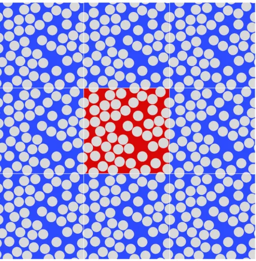
To analyze the transverse behavior of unidirectional FRPs, assuming infinitely long fibers, the microstructure can be idealized as a dispersion of circles of radius
r which represent the section of the fibers. This fiber distribution should be
rep-resentative of the actual transverse section microstructure of the studied material (Totry et al., 2010, 2009), many different methodologies have been proposed to at-tain this goal. Thus, there are techniques based on the replication of the images of the microstructure (Trias, 2005), on the reproduction of statistical spatial descriptors (t. J. Vaughan, 2011) or a direct technique which generates an idealized isotropic and random microstructure (Segurado and LLorca, 2002). The later technique was employed in this work to generate artificial microstructures of the FRPs, and the description of this method is given below.
The positions of the inclusions were created randomly and sequentially with the random sequential adsorption algorithm (RSA) (Segurado and LLorca, 2002). The fiber diameter,D, was determined from the total number of fibersN and the volume
fractionξ. The generation algorithm propose a center of fiber, i, which is accepted if
the distance between this fiber and all the fibers previously accepted j = 1, ..., i−1
exceeded a minimum value, 1.035D, imposed by the feasibility of creating an
ad-equate finite elements mesh. If the fiber i cuts any of the square unit cell sides,
the microstructure of the composite is periodic (Fig.1.6). If~x stands for the center
coordinates of circle ithese conditions are expressed by
minn||~xi−~xj+~h||o≥1.035D (1.7)
for any value of ~h = (k, l) where k and l can take the values 0, L,−L, leading to
5 conditions which should be checked for each pair of fibers. Moreover, to avoid distorted finite elements during meshing, the fiber surface should not be very close to the cell faces, and this led to an extra condition
||xik−r|| ≥0.045D ; k = 1,2 (1.8)
||xik+r−L|| ≥0.045D ; k = 1,2 (1.9)
Boundary conditions
The RVE together with the boundary conditions must generate valid tilings for the underformed and the deformed states. Thus, gaps or overlaps between neigh-boring cells and unphysical constraints should be avoided in the problem solution as they lead to continuum mechanics inconsistencies. In order to achieve this, the applied boundary conditions should generate the appropriate deformation modes for the studied load cases. The most commonly employed boundary conditions are the symmetry and periodicity.
Symmetric boundary conditions
Figure 1.7: Periodic square and hexagonal fiber arrangement and its units cells (Pettermann and Suresh, 2000).
Figure 1.9: Diagram of periodic boundary conditions in a rectangular two dimen-sional model.
Symmetric boundary conditions are typically very useful for describing simple microgeometries, they are fairly easy to use and have very low computational cost. However, the load cases that can be handled by symmetric boundary conditions are limited to homogeneous thermal loads, mechanical loads acting in directions normal to one or more pairs of faces, and combinations of them.
Periodic boundary conditions
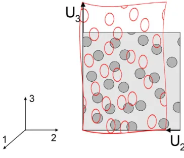
Periodic boundary conditions are considered the more general way to introduce a far-field stress and strain into the RVE. The application of periodic boundary conditions to the edges of the RVE ensures the continuity between neighboring RVEs, which deform like jigsaw puzzles (Fig. 1.9).
The periodic boundary conditions in a general three dimensional unit cell can be expressed in terms of the displacement vectorsU~1, ~U2 and U~3 between opposite faces
~u(0, x2, x3)−~u(L1, x2, x3) = U~1 (1.10)
~u(x1,0, x3)−~u(x1, L2, x3) = U~2 (1.11)
~u(x1, x2,0)−~u(x1, x2, L3) = U~3. (1.12)
where L1, L2 and L3 are the dimensions of the RVE along their coreresponding
di-rections.
Periodic boundary conditions can be used to introduce any physically homoge-neous deformation state within the unit cell. For example, a uniaxial tension along the x3 axis is imposed with U~3 = (0,0, δt), where δt stands for the imposed tensile
displacement. The components of U~1 and U~2 are chosen so that the all the normal
and shear forces acting on the RVE surfaces are zero (besides those corresponding to the imposed transverse tension). The corresponding logarithmic strain is given by
3 = ln (1 +δt/L3), and the corresponding Cauchy normal stress (σ3) can be
com-puted from the resultant normal forces acting on the RVE faces divided by the actual cross-section.
An important drawback of periodic boundary conditions is the high computa-tional cost when they are applied in a finite elements code because of the multipoint constraints required for their implementation.
1.6.2
Embedded cells
Figure 1.10: Schematic of an embedded cell approach to simulate the three-point bending test of a notched beam specimen.
is modeled in detail while the remaining beam is considered to be an homogeneous material.
Depending on the considered outer region, Böhm (1998) classified the embedded cell approaches in three basic types:
• Models which employ discrete microstructures for the core and the embedding regions, but discretized with different element size (Sautter et al., 1993). This model can easily reproduce a full sample with a refined mesh in some regions of interest, avoiding the usual layer effects produced at the interfaces between the core and the outer region. However, this strategy has an important drawback in the very high computational cost.
• Models which take into account the outer region as a homogeneous material with a constituve law defined a priori based on empirical or micromechanical approaches. These models are specially suited to study the localization and growth of cracks in inhomogeneous materials (Wulf et al., 1996; González and LLorca, 2007b) or the stress concentrations near the crack tips (Aoki et al., 1996) or around local defects (Xia et al., 2001).
scheme. In a first step, trial properties are impose to the outer region, the stress and strain fields are computed in the microstructure of the core. In the following steps, the homogeneous response of the core is used for the constitutive behavior of the outer region. This process is repeated until the convergence is achieved. These models have been mainly employed for material characterization (Yang et al., 1994; Chen, 1997). They are easily used in elastic regime, but they can be very complex when dealing with elastoplastic behavior.
1.7
Constitutive models for FRPs microconstituents
A critical issue in computational micromechanics is to account for the actual de-formation and failure micromechanisms of each phase and this is carried out normally through the appropriate constitutive equations at the constituent level. In the par-ticular case of unidirectional composites loaded in the transverse plane, the behavior under compression is controlled by the shear yielding of the matrix and the deco-hesion of the fiber-matrix interfaces. Moreover, under transverse tension loads the brittle decohesion of the interfaces triggers the final failure of the material, leading to a brittle behavior of the composite. The different processes have to be taken into account in the numerical analysis to provide realistic results.
network created between the prepolymers. Since the cross-linking is a nonreversible process, the shape of the created component cannot be changed after curing.
The most common polymeric matrices for high performance and aircraft grade composites are the epoxy resins. They have been extensively used due to their ex-cellent properties such as good adhesion, good corrosion resistance, low shrinkage and processing versatility. On the other hand, epoxy resins present some important drawbacks, such as their cost and higher viscosity than other thermosetting resins, which results in more intricate and costly manufacturing processes. Therefore, the epoxy is only employed in high added-value applications such as aircraft, sports, etc. The matrix-fiber interfaces of FRPs are widely studied in different fields. Chem-istry and molecular physics study topics as the nature of the bonds, surface density or their ranges of action at molecular level (Fowkes, 1987; Mittal, 1995). However, from a technical viewpoint, the most relevant problems of the interfaces are the stress transfer efficiency, their strength and the process of decohesion (see Fig. 1.11) (Zhan-darov and Mäder, 2005).
1.7.1
Plastic behavior of the matrix
The highly linked 3D network structure of a cured epoxy resin provides the solid material with outstanding mechanical properties. As any polymeric system, its initial deformation is dominated by the viscoelastic phenomena. However, due to the exten-sively entangled of its macromolecules, these time dependent effects can be neglected and modeled as an isotropic linear elastic solid until yielding.
The yield behavior of polymers depends on temperature and strain rate. However, the conventional yield criteria can accurately describe the plastic behavior of polymers by controlling the test conditions. Following this strategy, many studies of the yield behavior of epoxies have bypassed the question of strain rate and temperature and sought to establish a yield criterion (Cherry and Thomson, 1981; Kinloch and Young, 1983).
in these materials is often defined as the point of maximum load, at which that the subsequent deformation occurs without further increase in stress (Yee et al., 2000). Moreover, the yield behavior of epoxies is pressure-sensitive, and yield stress decreases with hydrostatic tension and increases with hydrostatic compression. This dependence is taken into account by pressure-dependent yield criteria like Mohr-Coulomb or Drucker-Prager, which were initially developed to characterize the plastic flow of soils and rocks.
Mohr-Coulomb yield criterion
The Mohr-Coulomb criterion assumes that yielding takes place when the shear stress acting on a specific plane, τt, reaches a critical value, which depends on the
normal stress,σn, acting on that plane. This can be expressed as
τt=c−σntanφ (1.13)
where c and φ stand, respectively, for the cohesion and the friction angle, two
ma-terials parameters which control the plastic behavior of the material. Physically, cohesion crepresents the yield stress under pure shear loading while the friction
an-gle takes into account the effect of hydrostatic pressure. Whenφ = 0◦ Mohr-Coulomb
model is reduced to the pressure-independent Tresca model while φ = 90◦ leads to
the “tension cut-off” Rankine model. The value of both parameters for an epoxy can be approximated from the strength,σyc, and the orientation of the shear bands,θ, in
uniaxial compression tests. They are given by
σyc = 2c cos φ
1−sinφ and θ = 45 +φ/2 (1.14)
where θ is the shear band angle, typically 50◦ < θ < 60◦ for uniaxial compression
loads in epoxy matrices (Puck and Schürmann, 2002; Pinho et al., 2006; Aragonés, 2007; Totry et al., 2008a).
The yield surface of the Mohr-Coulomb model can be rewritten in terms of the maximum and minimum principal stresses (σI and σIII)
Q
sc sc
sc
t
s
F
2Q
Figure 1.12: Shear band created by a uniaxial compression stress and Mohr’s circle for this stress state.
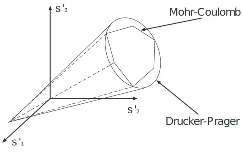
The Mohr-Coulomb criterion presents two important drawbacks for its practical application. First, it does not depend on the intermediate principal stress, σII,
which underestimates the yield strength of the material in many cases (Mogi, 1971). Second, the yield surface in Fig. 1.13 shows sharp corners which impairs its numerical implementation.
Drucker-Prager yield criterion
The criterion was initially proposed to deal with the plastic deformation of soils (Drucker and Prager, 1952). However, this yield criterion and its subsequent mod-ifications have been extensively applied to other pressure-dependent materials like rocks (Zhang and P. Cao, 2010), concrete (Arslan, 2007) or polymers (Quinson et al., 1997).
The linear Drucker-Prager yield function can be expressed as
FDP(J1, J02, α) = r
3
2J02+J1α−d = 0 (1.16)
where J1 is the first invariant of the stress tensor, J02 is the second invariant of the
Mohr-Coulomb
Drucker-Prager
s
'
3s
'
2s
'
1Figure 1.13: Mohr-Coulomb and Drucker-Prager yield surfaces in the deviatoric stress space.
andαis the pressure sensitivity parameter, which, according to experimental results,
is in the range 0.10-0.30 for glassy polymers (Kinloch and Young, 1983).
The Drucker-Prager yield criterion can also be rewritten in terms of the principal stresses, as in the case of the Mohr-Coulomb criterion,
FDP(σI, σII, σIII) =
r
(σI−σII)2+ (σII−σIII)2+ (σIII −σI)2
2
+ (σI +σII +σIII)α−d = 0 (1.17)
Interrelationship between Mohr-Coulomb and Drucker-Prager parameters
Mohr-Coulomb surface by the selection of the parameters α and d, through the
fol-lowing relations (Jiang and Xie, 2011)
α= −sinφ
cosη−(1/√3) sinηsinφ (1.18)
d= ccosφ
cosη−(1/√3) sinηsinφ (1.19)
whereηis the Lode angle, which is controlled by the relationship of the intermediate
principal stress and the major and minor principal stresses, providing different possi-bilities to match the Drucker-Prager and Mohr-Coulomb criteria (Fig. 1.14). If both surfaces match along the compressive meridian (η=−30◦), the Drucker-Prager cone
represents an outer bound cone of the Mohr-Coulomb hexagonal pyramid. When
η = 0◦ the surfaces match along shear meridian, and the inner cone of the
Mohr-Coulomb yield surface coincides with Drucker-Prager at η= 30◦.
1.7.2
Matrix damage behavior
The epoxy resins employed in the matrix of FRPs exhibit large deformations and plastic yielding under compressive loads, while tension stresses lead to sudden failure. The characterization of the fracture behavior of the matrix is an essential step to study the mechanical behavior of the FRPs.
D-P(h=30)
D-P(h=-30)
D-P(h=0) M-C
s
'
1s
'
3s
'
2the new area created during the crack propagation. Griffith introduced the concept
fracture energyof a materialGf, only applicable to perfectly brittle materials and the
experimental measurements of the energy necessary to propagate a crack were orders of magnitude higher than the theoretical estimations. Experimental observations of the crack surfaces showed that plastic deformation takes place at the notch of the tip, even for brittle materials. This led to Irwin (1948) and Orowan (1955) to adopt the concept of the fracture process zone for the region surrounding the crack tip. This
zone was characterized by a progressive softening, for which the stress decreases at increasing deformation. The fracture process zone is surrounded by a nonsoftening nonlinear region characterized by plasticity, for which the stress remains constant at increasing deformation. In addition, Irwin estimated the size of the fracture process zone through a parameter called characteristic length, which was defined by Hilleborg et al. (1976) as
lch= EGf
σt2
(1.20)
in which E is the elastic modulus and σt2 is the tensile strength of the material.
It is possible to distinguish between three types of fracture behavior depending on the ratio between the size of the structure and the characteristic length (D/lch)(Fig.
1.15).
Figure 1.15: Types of fracture process zone. Diagrams at the bottom show the trends of the stress distributions along the crack line. From Bažant and Planas (1998).
Epoxies fail in tension exhibiting very limited elongation and this brittle behavior has been classically treated by means of LEFM (Kinloch and Young, 1983). However, the theoretical fracture toughness, considering a perfectly brittle material, usually underestimates the experimental measurements (Berry, 1964). This fact has been confirmed by fractografic observations were massive plastic deformations by shear banding and crazing around the crack tip were observed (Patrick, 1973). These findings confirmed that toughening mechanisms are operating during the fracture of the epoxy resin and they can be also treated as quasibrittle materials. The fracture
process in these materials can be properly described by two simplified approaches: cohesive crack models and continuum damage models.
Cohesive crack models
~
~ ~~
real crack cohesive crack continuum damage
(b) (a) s s s stress, s
elongation, DL microcracks
Figure 1.16: Real rough crack idealized as a cohesive crack and a continuum damage model. Stress-elongation curve for the idealized stable tension test.
Fang et al., 2011). In this model the entire fracture process zone is lumped into the crack line and is characterized in the form of a stress-displacement law which exhibits softening (Fig. 1.16(a)). Thus, a cohesive crack is a fictitious crack able to transfer stresses from one face to the other, according to a softening function which is considered a material property. The cohesive crack can be implemented in finite elements codes by means of different methods like extended finite elements, cohesive elements, strong embedded discontinuities, etc. These strategies have been employed to simulate the fracture behavior epoxy resins (Diehl, 2008; Campilho et al., 2011; Y. T. Kim, 2011).
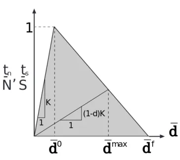
The progressive interface fracture upon loading can be taken into account through the cohesive crack model at the interface between dissimilar materials (Camanho and Dávila, 2002; Segurado and LLorca, 2004). The mechanical behavior of the cohesive crack was expressed in terms of a traction-separation law which relates the displacement jump across the interface with the traction vector acting on it. The initial response of the cohesive elements is linear in absence of damage. Therefore, for a two dimensional cohesive element, the traction-separation law could be written as
wheretn,ts,δnandδs stand for the normal and tangential tractions and displacement
jumps across the interface respectively. The linear behavior ends at the onset of damage, which is dictated by a maximum stress criterion expressed mathematically as
max{htni
N , ts
S}= 1 (1.22)
in whichhi stand for the Macaulay brackets indicate that does not develop when the
interface is under compression. N and S are the normal and tangential interfacial
strengths, respectively. Once damage begins, the stress transferred through the crack is reduced depending on the interface damage parameterd, which evolves from 0 (in
the absence of damage) to 1 (no stresses transmitted across the interface), as shown in Fig. 1.17. The corresponding traction-separation law is expressed by
tn = (1−d)Kδn if δn>0
tn = Kδn if δn≤0 (1.23) ts = (1−d)Kδs
For a linear softening law, the evolution of the damage parameter is controlled by an effective displacement, ¯δ, defined as the norm of the displacement jump vector
across the interface as
¯
δ=p< δn >2 +δs2, (1.24)
andddepends on the maximum effective displacement at the interface attained during
the loading history at each material integration point ¯δmax according to
d = δ¯
f(¯δmax−δ¯0)
¯
δmax(¯δf −δ¯0) (1.25)
where ¯δ0 and ¯δf stand for the effective displacement at the onset of damage (d= 0)
t t
N S
,
-n s
1
d
d
0d
maxd
f1
(1-d)K 1
K
Figure 1.17: Schematic of the traction-separation law governing the behavior of the cohesive crack at the fiber/matrix interface.
model, the energy necessary to completely break the interface is the interface fracture energy G, which can be defined as
G= 1
2Tef fδf (1.26)
being Tef f the effective traction at the damage initiation
Tef f = √
N2+S2 (1.27)
Continuum damage models
elements codes through the degradation of the elastic moduli, the decreasing of the yield stress or combining both. The different approaches have a similar response upon the material loading, but differences appear during the unloading (Fig. 1.18).
The first continuum damage model was proposed by Kachanov (1958) and Rabot-nov (1968) by introducing a scalar internal variable to take into account the reduction of the cross-sectional area produced by microcracking during the creep failure in met-als. Therefore, denoting respectively byAo and A the effective load bearing areas of
the pristine and damage material, the damage variable,DK, was introduced by
DK =
A−Ao
A (1.28)
where DK = 0 represents undamaged material and DK = 1 fully damaged material
with a total loss of load-bearing capacity. Considering the damage variable, the observed stress, σ, is replaced by the effective stress, σef f.
σef f = σ
1−D (1.29)
Lemaitre (1984) also considered a scalar damage variable, DL, to represent the
stiffness degradation experimentally observed in ductile metals under load-unload cycles
E = (1−DL)Eo (1.30)
The damage evolution can also be coupled with the plastic behavior of metals, Gurson (1977) described the mechanism of damage by void growth in porous metals producing an evolution of the yield surface. Initially, when the material is undamaged
DG = 0, the plastic behavior is governed by the von Mises yield criterion. However,
in presence of damage, DG 6= 0, the yield behavior becomes pressure-sensitivity and
the yield surface shrinks.
strain,
e
stress,
s
Eo
E=(1-D)Eo
strain,
e
stress,
s
Eo
Eo
Figure 1.18: Illustration of loading-unloading curve for the smeared crack model implemented through the degradation of the elastic moduli and the decrease of the yield stress.
et al., 2009) or FRPs (Ladevèze and Lubineau, 2001; Camanho et al., 2007; Maimí et al., 2007).
Strain localization and mesh adjustment
When the crack opening is modeled by a displacement jump, as it is done by the cohesive crack models, it is possible to formulate an objective traction-separation law. In this case, the numerical result does not exhibit pathological mesh sensitivity. On the other hand, when the crack is smeared over a softening region of an arbitrary size (e.g. the element size), the resulting model can be physically incorrect and numerically ill-posed.
For illustrating this problem, let us consider a homogeneous bar of initial length L subjected to a tensile load and made of softening material. This bar can be subdivided inN identical pieces which act as equal elements coupled in series. In this case, after
strain,
e
stress,
s
s
1 2 3
. .
.
.
NL
N = 1
N = 2
N = 3
N = 4 N = 8
Figure 1.19: Homogeneous bar subdivided intoN equal elements and the result-ing stress-strain curves.
(Fig. 1.19). This problem is referred as lack of mesh objectivity or spurious mesh sensitivity.
The mesh sensitivity is not acceptable in finite elements calculations and it must be avoided. The simplest remedy, frequently used in engineering applications, is based on an adjustment of the stress-strain diagram depending on the size of the element. This technique was proposed for softening plasticity models (Pietruszczak and Mroz, 1981) and later applied to damage models (Bažant and Oh, 1983). The degradation of the material is due to the opening of microcracks which later collapse into a macroscopic crack producing the final failure. If the crack opening is modeled by a displacement discontinuity, as is done in the cohesive crack models, it is possible to formulate a traction-separation law as the constitutive description of the damage. Since the crack opening does not depend on the element size, the numerical results do not exhibit pathological mesh sensitivity because the physical description of the fracture process is objective. Then, a stress-strain law can be constructed at each material point by taking into account the width of the simulated process zone (which depends on the type and size of the corresponding finite elements).
σn=f(w) (1.31)
where σn is the traction stress perpendicular to the crack plane and w is the crack
opening. Considering for simplicity a uniaxial problem (σn = σ), if the crack is
smeared over a distanceh, the resulting cracking strain is
crack = w
h =
f−1(σ)
h (1.32)
The total strain in the localization region (Ls) is obtained by combining the
cracking and the elastic strains
=elastic+crack = σ
E +
f−1(σ)
h (1.33)
The remaining part of the material (Lu = L−Ls) is in elastic regimen and its
strain is given byelastic. Thus, the total elongation of the material is
u=Luelastic+Ls(elastic+crack) =Lelastic+Lscrack = Lσ
E +
Ls h f
−1(
σ) (1.34)
WhenLs =h, the term corresponding to the crack opening becomes independent
of the finite elements discretization. Therefore, to avoid the mesh sensitivity it is necessary to obtain the value of Ls from the mesh characteristic length and set h
equal to this value. In uniaxial problems Ls is the size of the element, but the
selection of this parameter can be difficult in multidimensional problems or second-order elements (Oliver, 1989).
1.7.3
Damage-plasticity coupled model of the matrix
The cracking process in quasi-brittle materials is not a sudden onset of new free surfaces, but a continuous nucleation and coalescence of microcracks (Kinloch and Young, 1983; Metha and Monteiro, 1993) and the evolution of microcrack density produces a macroscopical softening in the material.
model employees a modification of the Drucker-Prager yield function to account for the different strength under tension and compression stress states. In terms of the invariants of the stress tensor,J1 and J20, the yield function is given by
FQB(J1, J02, σI, β, α) =
r
3
2J02+J1α+βhσIi −d(˜plc) = 0 (1.35)
where σI is the maximum principal stress and β is a function of the tensile and
compressive yield stresses,σt(˜plt ) and σc(˜plc) respectively, it is given as
β = σc(˜ pl c) σt(˜plt )
(1−α)−(1 +α) (1.36)
In many cases, it is useful to avoid the use of the cohesiondby rewriting the yield
function in term of the compression yield stress
FQB(J1, J02, σI, β, α) =
1 1−α
r
3
2J02+J1α+βhσIi
!
−σc(˜plc) = 0 (1.37)
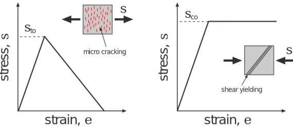
the yield surface under plane stress conditions is plotted in Fig.1.20. For compression stress states, the quasi-brittle material yields following the standard Drucker-Prager yield criterion. However, under tension loads, the criterion predicts a yielding mainly controlled by the maximum principal stress, similar to the Rankine model applied for perfectly brittle materials. The model assumes two competing deformation mech-anisms: the tensile cracking and compressive shear banding. The evolution of the yield surface is controlled by two internal damage variables ˜plt and ˜plc, depending on
the failure mechanisms under tension and compression loading, respectively.
Under uniaxial compression the response of the material is linear and elastic until the value of the initial yield σc0 which corresponds with the onset of the plastic
regime. For uniaxial tension, the stress-strain response follows a linear behavior until the value of the failure stress σt0 is reached. The failure stress corresponds to the
s
s
s
ts
cs
ts
cDrucker-Prager
Damage plasticity for quasi-brittle materials
I II
Figure 1.20: Yield surfaces in plane stress.
strain,
e
stress,
s
strain,
e
stress,
s
s
cos
s
shear yielding micro cracking
s
to1.7.4
Fiber-matrix interface
Matrix-reinforcement decohesion is one of the main damage mechanisms in FRPs because it leads to significant reductions of the strength, ductility and toughness of the material (LLorca, 2000). Interface fracture initiates by the nucleation of a crack as the stress at the interface exceeds the interfacial strength. Damage progresses as the crack propagates along the matrix-fiber interface and reduces the amount of load transferred from the matrix to the reinforcement. Finally, the fracture of the composite can occur by the coalescence of interface cracks connected by shear bands in the matrix. For these reasons, the fiber-matrix decohesion is considered a key mechanism which should be taken into account to analyze the overall composite behavior.
Interface fracture in composites has been modeled by two different strategies. Mean-field approximations (Zhao and Weng, 1996; Sun et al., 2003) represented the composite as a three-phase material formed by the continuous matrix, intact and debonded reinforcement. It was assumed that interface fracture was strength-controlled, and that decohesion occurred when the average tensile stress in the rein-forcement along the loading axis surpassed a critical value identified as the interface strength. These models provided the first estimations of damage evolution by in-terface fracture during deformation but present some limitations. First, inin-terface fracture is controlled by maximum stress values which may be very different from the average stress in the reinforcement. Second, they assumed that the interface decohe-sion was complete, while experimental observations always showed partial decohedecohe-sions (Fig. 1.11).
elasto-plastic deformation (Böhm and Han, 2001; Segurado et al., 2003; González et al., 2004).
1.8
Objectives
FRPs present outstanding mechanical properties (stiffness and strength) and low density, which compete favorably with metallic alloys, the standard structural mate-rials for engineering applications. Since FRPs became affordable, as a result of the maturation of the processing and quality control techniques, their use in structural components was spread in many industrial sectors. The strength of a composite lami-nate is assessed nowadays through the application of physically-based phenomenolog-ical failure criteria. These criteria establish a failure locus in the stress space, which is formed by the intersection of various smooth surfaces, each one representing the critical condition for a given fracture mode. However, the comparison of their pre-dictions with the experimental results indicate that the existing knowledge on failure mechanisms of FRPs needs further development. Therefore, without accurate models to predict the failure strength of laminates, it is necessary to perform a high number of tests to validate the safety of composite structures through a costly trial-and-error approach.
Recent developments in computational micromechanics have demonstrated that the mechanical behavior until fracture of a composite lamina can be obtained, know-ing the mechanical properties of its constituents, from numerical simulations of the composite microstructure. This can be the first step in a new multiscale modeling strategy aimed to predict the strength of composite structures. Nevertheless, to per-form this virtual testing strategy successfully it is necessary to gain a substantial knowledge of the mechanical properties of the FRPs constituents (matrix, fiber and interfaces) and the failure mechanisms developed in the microstructure. Thus, the objectives of this thesis can be identified as follows.
processes occurring at the microscale. For this reason the second goal of this work is the detailed experimental characterization of a glass fiber/epoxy laminate, where the most relevant mechanical properties of the matrix and the fiber/matrix interfaces
were obtained by means of nanoindentation and push-out tests. Moreover, additional information about the deformation and damage mechanisms at the micron scale was obtained through the application of in situ SEM testing carried out on cross-section
Characterization of the transverse
properties of unidirectional FRPs
The compressive and tensile mechanical properties of a commercial unidirectional laminate of epoxy-matrix reinforced with glass fibers were determined, in the trans-verse direction, by means of the ASTM standard test methods.
2.1
Material
Unidirectional laminates ([0]14) were manufactured from pre-impregnated sheets
of E-glass/MTM 57 epoxy resin (Advanced Composite Group, UK). Rectangular panels of 350 x 300 x 2.5 mm3 were heated at 3◦C/min and consolidated at 120◦C
under 0.64 MPa of pressure in an autoclave for 30 min. They were cooled at the same rate of 3◦C/min and the pressure was released at 80◦C. After manufacturing,
2.5mm
4.5mm 25mm
140mm 10mm
Tabs
Gage section
1 2
3
1 2
3 2
Figure 2.1: Schematic picture of the transversal compression test specimens.
2.2
Compressive properties determination
The transverse compressive properties of the unidirectional E-glass/MTM 57 epoxy laminate were determined according to the ASTM D 3410 standard test method. This test procedure introduces the compression into the specimen through shear forces acting throughout the grips. The compression specimens were machined from the panels of unidirectional laminate with the dimensions recommended by the ASTM standard (Fig. 2.1). Tabs of woven E-glass FRPs were employed to prevent the premature failure of the specimen in the grip area. The tabs were bonded to the specimen surface with an epoxy adhesive, leaving 10 mm of free gage length between them.
as-semblies are attached to the crosshead of the testing machine. Tests were carried out in a servo-hydraulic mechanical testing machine Instron 8803, under stroke control using a constant cross-head speed of 1mm/min while the load and the displacement were measured using a 25kN Instron load cell and the displacement transducer of the mechanical rig, respectively. The transversal strain was measured using a digital image correlation technique (Vic, Correlated Solutions, Inc.). To this end, one of the specimen surfaces was painted in white and then sprayed in black to created a ran-dom pattern of black dots over the white background. The digital image correlation system acquired a high-resolution image of the surface every 2 s and tracked the dis-placement of the black dots to create a map of the disdis-placement field on the specimen surface. The local lagrangian strain tensor was computed directly as the derivative of the interpolated displacement field obtained from the digital image correlation sys-tem. Further details on this measurement technique are described in Chapter 5. In addition, some of the specimens were instrumented with 350 Ω strain gages at both sides to monitor the degree of bending introduced and to check the accuracy of the optical strain method. The strains measured by the strain gages were equivalent to that obtained by the digital image correlation until the strain gages were detached form the specimen.
2.2.1
Experimental results
Ten transversal compression tests were performed on unidirectional [0]14 E-glass
/ MTM 57 coupons according to the ASTM 3410 standard. The stress-strain curves (σ2 −2) are plotted in Fig. 2.3. The stresses were computed from the readings of
the load cell and the initial cross sectional area of the specimen, while the digital image correlation system allowed the measurement of full-field deformations. The tests were reproducible and exhibited a limited experimental scatter. The shape of the stress-strain curves was typical of unidirectional polymer composites subjected to transversal compression. The behavior was initially linear and the slope of the curve was used to compute the transverse elastic modulus of the laminateE2 ≈12±2 GPa.
ALIGNMENT
RODS
CLAMPING
SCREWS
TABBED
SPECIMEN
LINEAR
BEARINGS
LOAD-ALIGNMENT
BLOCK
0 50 100 150 200
0 1 2 3 4 5
σ 2
(MPa)
ε2 (%)
Figure 2.3: Transverse compressive stressvs. strain curves for E-glass/MTM 57 epoxy specimens.
of the decohesion of the fibers. In turn, this region ended with the catastrophic failure of the laminate. The strength of the material was obtained, according to the ASTM standard, as the ultimate load divided by the cross sectional area of the specimen, which provided a value ofYc≈160±10 MPa
Fracture surfaces were visually inspected after the compression tests. In all cases, the fracture plane was parallel to the fiber direction and perpendicular to the trans-verse plane 23, which is an acceptable failure mode according to ASTM standard. Due to the short gage length of the specimens, the failure was mostly located near the tab region, but never inside the grip portion of the specimen, which also meets the requirements of the Standard. The fracture surface of one of the tested coupon is shown in Fig. 2.4. The angle between the fracture plane and the direction per-pendicular to the loading axis was also measured by optical microscopy leading to a value of Θ≈54±2.0◦.
fracture processes of FRPs have pointed out that the fracture plane orientation of the composite under transverse compression can be mainly determined by the pres-sure sensitivity of the matrix. During the test, before the maximum compressive load is attained, shear bands of severe plastic deformation appear in the matrix. These bands are tilted at a certain angle with respect to the plane perpendicular to the loading axis and their orientation is dependent on the pressure sensitivity of the polymer. The deviation of the experimental fracture angle with respect to the maximum shear stress directions at±45◦ is indicative of the hydrostatic pressure
de-pendent yielding of the polymer matrix (González and LLorca, 2007a). Continuing with the compressive loading of the laminate, the damage by interface decohesion is developed afterwards around the shear bands. The final fracture occurs by the link-up of interface decohesions through the matrix, following the path previously set by the shear bands.
The previously described failure mechanism indicates that the fracture plane ori-entation is approximately given by the oriori-entation of the shear bands of the polymeric matrix. Therefore, the experimental measurement of direction of the failure plane provides an estimation of the pressure sensitivity parameter of the epoxy matrix. Considering that the plastic behavior of the matrix is represented adequately by a non-dilatant Drucker-Prager yield model, the orientation of the shear bands is given by (Rudnicki and Rice, 1975; Gao et al., 2011)
Θ = tan−1 s
ζ−Nmin Nmax−ζ
(2.1)
whereζ = (1 +ν)(α)−N(1−ν), Nmax = σ0
I
¯
τ , N = σ0
II
¯
τ , Nmin = σ0
III
¯
τ , ¯τ =σmises/ √
3, beingν the Poisson ratio andαthe pressure sensitivity in the Drucker-Prager model.
Following this strategy, the measured orientation of the fracture plane Θ ≈ 54
represents a pressure sensitivity parameter of α ≈ 0.13 in the Drucker-Prager yield