Economic impact of freer trade in Latin America and the Caribbean : a GTAP analysis

Texto completo

(1)V.  N.  (NOVEMBER, ), –. ECONOMIC IMPACT OF FREER TRADE IN LATIN AMERICA AND THE CARIBBEAN: A GTAP ANALYSIS* KAKALI MUKHOPADHYAY** PAUL J. THOMASSIN*** DEBESH CHAKRABORTY**** The recent worldwide economic conditions resulting from the financial crisis call for greater cooperation. This paper assesses the impact of trade reforms between Latin America and the Caribbean (LAC) and India and LAC and the EU (European Union) at 2020 using a global computable general equilibrium (CGE) model. The findings show that LAC-EU tarif f reduction appears to be beneficial for both regions in the short run, though not so in the long run, while the LAC-India tarif f reduction impact appears to be more beneficial for both economies in the long run. This important finding emphasizes the scope and opportunities for south-south cooperation in the long run. JEL classification: F15, F18, C68 Keywords: Latin America and the Caribbean, European Union, India, Global Trade Analysis Project (GTAP). 1.. INTRODUCTION. Latin American and Caribbean countries have grown rapidly in recent decades. However, this growth stretch has been hampered by the worldwide financial crisis of the past few years. The impacts of this crisis have been transmitted to the region mainly through the channels of external trade and export prices (Economic Commission for Latin America and the Caribbean - ECLAC, 2009). After growing continuously for six years, the gross domestic product (GDP) of Latin America and the Caribbean declined by 1.8% in 2009, resulting in increased unemployment and poverty (ECLAC, 2009). * This is a revised version of a paper presented at the 3rd Regional Meeting on Computable General Equilibrium (CGE) Modeling organized by The Inter-American Development Bank (IDB) and the Economic Commission for Latin America and the Caribbean (ECLAC), held at the Institute for the Integration of Latin America and the Caribbean (IDB-INTAL) in Buenos Aires, Argentina, in September 2010. The authors are grateful to the meeting participants for their valuable comments and suggestions. The authors would also like to thank the reviewers for their comments on the manuscript. ** Corresponding author. Department of Agricultural Economics, McGill University, MacDonald Campus, 21,111 LakeShore, Ste Anne De Bellevue, Montreal, Québec, Canada. E-mail: kakali.mukhopadhyay@mcgill.ca. *** Department of Agricultural Economics, McGill University. **** Department of Economics, Jadavpur University, Kolkata, India.. DOI 10.7764/LAJE.49.2.147.

(2) 148. LATIN AMERICAN JOURNAL OF ECONOMICS | V.  N.  (N, ), –. The financial crisis af fected the region’s trade, with Latin America’s worldwide exports declining 31% in the first half of 2009. According to ECLAC estimates, the volume of regional trade shrank by approximately 13% in 2009, more than the 10% decline projected for global trade, while the volume of exports and imports for the Latin American and Caribbean region dropped significantly. The crisis has also af fected investment and private consumption (ECLAC, 2009). After contracting in 2009, GDP expanded by 5.9% in Latin America and the Caribbean in 2010, although performance varied significantly among countries in the region. This expansion was caused by strong domestic demand in the forms of consumption and investment, and also by buoyant external demand (ECLAC, 2010-11). On the domestic demand side, private consumption growth (up 5.9%) occurred because of an improvement in employment and wages. Public consumption rose at a modest rate of 3.9%. Investment grew by 14.5%, with strong growth in the machinery and equipment segments in particular. On the external demand side, exports of goods and services rose by over 10%. On the other hand, imports increased by more than 10%. For 2012, ECLAC projects regional growth of 4.1%, equivalent to a 3.0% rise in per capita GDP, notwithstanding the downturn in external conditions. Developed economies are likely to grow by 2.4% in 2012 (ECLAC, 2010-11). Meanwhile, the economic recovery is likely to be fragile in the United States and Japan, and Europe’s economy is projected to grow by just 1.9% in 2012. Developing economies will be the major players in global growth, with a rate of 6.2% projected in 2012. The strongest performers are expected to be China (8.9%) and India (8.2%) in 2012 (ECLAC, 2010-11). These new international conditions call for greater regional cooperation, not only to contain the adverse impact of the crisis but also to improve the region’s position in the global economy. In this sense, Latin American and Caribbean countries need to adopt a more coordinated approach to tightening ties with Asia-Pacific countries (ECLAC, 2010). Besides the Asia-Pacific region, closer links with developed countries, particularly the European Union, would likely benefit the LAC region in terms of addressing the current crisis. The LAC-EU summit in Peru in 2008 and recently in Madrid in 2010 are evidence of attempts to strengthen LAC-EU coordination and cooperation. Towards this end, this paper makes a modest attempt to study the impact of economic cooperation between the LAC region and other countries..

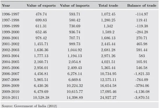
(3) K. Mukhopadhyay, P.J. Thomassin, and D. Chakraborty | FREER TRADE IN LAC. 149. Specifically, the objective of the study is to evaluate the economic impacts of freer trade between LAC and India, and LAC and the EU. The rest of the paper is organized as follows. Section 2 briefly reviews the efforts already in place between LAC-India and LAC-EU. Section 3 develops the method of analysis. The data, aggregation scheme, scenario development and macro variable assumptions are presented in Section 4. Section 5 discusses the results. Section 6 concludes the paper.. 2.. A BRIEF REVIEW OF INITIATIVES. LAC countries have entered into a significant number of trade agreements with countries around the world. These include around 90 trade agreements, of which 55 are FTAs and more than 40 are partial preferen tial trade agreements. Of the 55 FTAs, 21 are between LAC countries and the EU or Asian economies, while the rest mainly address integration among LAC countries (for details, see Appendix B).. 2.1. Ef forts made by LAC-INDIA Several Latin America and Caribbean countries and the government of India are working on ways to augment trade and commerce between India and LAC countries and are encouraged by the fact that trade relations between India and the region have grown in recent years. Trends in Indian exports and imports are shown in tables 1 and 2. North America and Europe have continued to be important destinations for Indian products, although their combined share declined from 46.2 to 29% from 2002-03 to 2010-11. On the other hand, the share attributed to Asia, including ASEAN, steadily increased from 2002-03 to 2010-11 (4 to 56%). Exports to Latin America are on the rise. On the import side, Asia’s share was around 61% in 2010-11, while the share of North America and Europe together has declined from 31 to 18%. As shown in Table 3, India’s trade with Latin American countries during the last few years has been growing steadily, increasing from US$1.07245 billion in 1996-97 to US$24.927 billion in 2010-11. India’s exports totaled US$10 billion and imports reached US$14 billion in 2010-11, resulting in an unfavorable balance of trade. In Latin America, Brazil was the main destination for Indian exports, followed by Mexico, Colombia and Argentina. Chile is the top exporter to India, followed by Brazil and Argentina. In terms of products, chemicals.

(4) 21.99. North America. 100. Total. Source: Government of India (2012). 100. 35.04. Rest of the world. 1.70 30.12. Latin America & the Caribbean. Asia. 8.16. 24.98. Europe. North America. 2002-03. Total. 100. 6.89. 47.60. 1.78. 19.19. 24.54. 2003-04. 100. 30.70. 35.36. 1.53. 7.37. 24.04. 2003-04. 100. 32.03. 36.18. 1.84. 6.97. 22.98. 2004-05. 100. 6.85. 49.50. 2.58. 17.52. 23.55. 2004-05. Trends in Indian imports (% share). Region. Table 2.. Source: Government of India (2012). 6.99. 44.39. Rest of the world. Asia. 2.46. 24.17. Europe. Latin America & the Caribbean. 2002-03. Trends in Indian exports (% share). Region. Table 1.. 100. 34.51. 34.58. 1.79. 6.96. 21.18. 2005-06. 99.98. 6.72. 48.38. 2.90. 17.82. 24.16. 2005-06. 100. 8.26. 57.51. 3.18. 7.41. 23.64. 2006-07. 99.97. 8.07. 49.78. 3.38. 15.85. 22.89. 2006-07. 100. 12.60. 59.69. 2.98. 9.15. 15.59. 2007-08. 100. 9.99. 51.68. 3.61. 13.49. 21.23. 2007-08. 100. 13.10. 62.06. 3.55. 6.92. 14.38. 2008-09. 100. 10.94. 52.04. 3.45. 12.21. 21.37. 2008-09. 100. 15.56. 60.81. 3.67. 6.61. 13.34. 2009-10. 100. 10.68. 53.95. 3.61. 11.55. 20.21. 2009-10. 100. 16.93. 61.16. 3.89. 5.97. 12.05. 2010-11. 100. 10.30. 56.10. 4.19. 10.72. 18.69. 2010-11. 150 LATIN AMERICAN JOURNAL OF ECONOMICS | V.  N.  (N, ), –.

(5) 151. K. Mukhopadhyay, P.J. Thomassin, and D. Chakraborty | FREER TRADE IN LAC. and pharmaceuticals were the leading exports from India, followed by engineering products. Copper accounted for around 90% of Chile’s exports to India, while vegetable oils formed approximately 80% of Argentine exports to India (Focus: LAC, 2008). Table 3.. India’s trade with Latin American countries. (US$ millions) Year. Value of exports. Value of imports. Total trade. Balance of trade. 1996-1997. 478.74. 593.71. 1,072.45. -114.97. 1997-1998. 699.83. 580.42. 1,280.25. 119.41. 1998-1999. 611.31. 730.69. 1,342. -119.38. 1999-2000. 652.46. 936.74. 1,589.2. -284.28. 2000-2001. 978.42. 707.71. 1,686.13. 270.71. 2001-2002. 1,455.71. 989.73. 2,445.44. 465.98. 2002-2003. 1,636.36. 1,044.92. 2,681.28. 591.44. 2003-2004. 1,777.13. 1,194.13. 2,971.26. 583. 2004-2005. 2,160.71. 2,054.8. 4,021.51. 105.91. 2005-2006. 2,956.01. 2,409.43. 5,365.44. 546.58. 2006-2007. 4,456.81. 6,278.14. 10,734.95. -1,821.33. 2007-2008. 5,905.51. 6,669.6. 12,575.11. -764.09. 2008-2009. 6,430.26. 10,224.32. 16,654.58. -3794.06. 2009-2010. 6,479.69. 10,615.77. 17,095.46. -4,136.08. 2010-2011. 10,528.38. 14,398.89. 24,927.27. -3,870.51. Source: Government of India (2012). A series of recent initiatives have been implemented to foster the trade relationship between India and LAC; these initiatives are summarized below (Focus: LAC 2008).. Preferential trade agreement with MERCOSUR India and MERCOSUR1 signed a framework agreement in June 2003 in Asunción, Paraguay. As a follow-up to the framework agreement, a preferential trade agreement (PTA) was signed in New Delhi in January 2004 with a view to expanding and strengthening the relationship between MERCOSUR and India and promoting trade. 1. MERCOSUR: Brazil, Argentina, Paraguay, Uruguay and Venezuela..

(6) 152. LATIN AMERICAN JOURNAL OF ECONOMICS | V.  N.  (N, ), –. expansion through reciprocal fixed tarif f preferences with the ultimate objective of creating a free trade area between the parties. The India-MERCOSUR PTA contains five appendices, which were signed in March 2005. The five appendices are the MERCOSUR Offer List, India Offer List, Rules of Origin, Safeguard Measures and the Dispute Settlement Procedure. Under this PTA, India and MERCOSUR have agreed to tariff concessions ranging from 10 to 100% on 450 and 452 tariff lines respectively. The major product groups covered in the MERCOSUR offer are food preparations, organic chemicals, pharmaceuticals, essential oils, plastics and articles thereof, rubber and rubber products, tools and implements, machinery items, electrical machinery and equipment. The major products included in India’s offer list are meat and meat products, inorganic chemicals, organic chemicals, dyes and pigments, rawhides and skins, leather articles, wool, cotton yarn, glass and glassware, iron and steel articles, machinery items, electrical machinery and equipment, and optical, photographic and cinematographic devices.. Preferential trade agreement with Chile India and Chile signed the Framework Agreement to Promote Economic Cooperation in January 2005. As a follow-up to the framework agreement, a PTA was finalized after four rounds of negotiations between the two sides, with the last round taking place in New Delhi in November 2005. The PTA has two appendices related to the list of products for which the two sides have agreed to set fixed tariff preferences and three appendices relating to rules of origin, preferential safeguard measures and dispute settlement procedures. While India has of fered to provide fixed tarif f preferences ranging from 10 to 50% on 178 tarif f lines at the eight-digit level to Chile, the latter has of fered India a similar range of tarif f preferences on 296 tarif f lines at the eight-digit level. The products on which India has of fered tarif f concessions include meat and fish products (84 tarif f lines), rock salt (1 tarif f line), iodine (1 tarif f line), copper ore and concentrates (1 tarif f line), chemicals (13 tarif f lines), leather products (7 tarif f lines), newsprint and paper (6 tariff lines), wood and plywood articles (42 tariff lines), some industrial products (12 tarif f lines), shorn wool and noils of wool (3 tarif f lines) and other products (7 tarif f lines). Chile’s offer covers certain agriculture products (7 tariff lines), chemicals and pharmaceuticals (53 tariff lines), dyes and resins (7 tariff lines), plastic, rubber and miscellaneous chemicals (14 tariff lines), leather.

(7) K. Mukhopadhyay, P.J. Thomassin, and D. Chakraborty | FREER TRADE IN LAC. 153. products (12 tariff lines), textiles and clothing (106 tariff lines), footwear (10 tariff lines), certain industrial products (82 tariff lines) and other products (5 tariff lines). The Agreement was signed in March 2006.. Institutional mechanisms The following institutional arrangements are already in place: (a) the Indo-Argentine Joint Commission; (b) the Indo-Argentine Joint Trade Committee; (c) the Indo-Mexican Joint Commission; (d) the IndoBrazilian Commercial Council; (e) the Indo-Cuban Joint Commission; (f) the Indo-Cuban Trade Revival Committee; (g) the Indo-Suriname Joint Commission; and (h) the Indo-Guyana Joint Commission.. 2.2. Ef forts made by LAC-EU The countries of Latin America and the Caribbean are taking concrete steps to diversify their economies and expand their markets in Europe. The EU and LAC are natural allies given their close historical, cultural and economic ties, as well as the increasing convergence of their basic values and principles (European Union, 2008). Building on this longstanding relationship between the two regions, the EU has established and strengthened links with LAC since the 1960s. In 1999, representatives of the EU and LAC met in Rio de Janeiro to form a strategic partnership aimed at fostering political, economic and cultural links between the two regions. The summit in Rio de Janeiro was followed by several biannual summits held in Madrid, Spain (2002); Guadalajara, Mexico (2004); Vienna, Austria (2006); Lima, Peru (2008); and recently in Madrid (Madrid Declaration, 2010). These events have facilitated the deepening of EU-LAC relations, reaffirming the regions’ commitment to promoting and strengthening their strategic partnership based on common principles, values and interests (European Union, 2008). The EU and Brazil launched their strategic partnership at the first EU-Brazil Summit in Lisbon in July 2007. In December 2007 the European Commission initiated an Economic Partnership Agreement (EPA) with the CARIFORUM2 countries (European Union MEMO/08/303). The EPA fully opens the EU market to Caribbean 2. CARIFORUM countries: Antigua and Barbuda, Bahamas, Barbados, Belize, Dominica, the Dominican Republic, Grenada, Guyana, Haiti, Jamaica, Saint Lucia, Saint Vincent and the Grenadines, Saint Christopher and Nevis, Surinam, and Trinidad and Tobago..

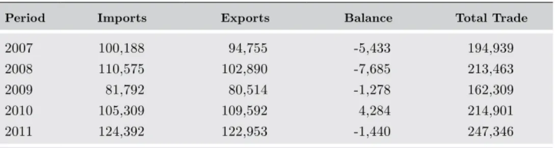
(8) 154. LATIN AMERICAN JOURNAL OF ECONOMICS | V.  N.  (N, ), –. exports and gradually opens the Caribbean market to new trade from the EU. Both Mexico (2000) and Chile (2003) have signed free trade agreements with the EU covering trade and investment. The Madrid Summit, which brought together heads of state and other government leaders from Latin America, the Caribbean and Europe, as well as important non-state actors, resulted in a decision to relaunch negotiations for an EU-MERCOSUR Free Trade Agreement and provide political approval for a comprehensive trade agreement between the EU and the Andean countries (Peru and Colombia) as well as the endorsement of the conclusion of negotiations between the EU and Central America3 (Madrid Declaration, 2010). The EU is Latin America and the Caribbean’s second-largest trading partner. Moreover, LAC’s trade with the EU has increased substantially since 1980, particularly during the last decade, resulting in trade figures that more than doubled between 1990 and 2008 (reaching approximately €180 billion in 2008) (European Union 2010, European Union 2008a). In 2006, the EU imports from LAC totalled €75 billion, and exports to the region amounted to €71 billion. Bilateral trade between the two regions amounts to around €160 billion annually (European Union MEMO/08/286). In 2007, the EU received around 14% of Latin American exports and 19% of Caribbean exports and these numbers continue to rise (European Union 2008b). Table 4 provides figures for the EU’s recent trade with LAC countries. The balance of trade is always negative from the EU’s standpoint except in 2010, which shows a large surplus. Table 4.. EU members states’ trade with LAC countries. (in millions of euros) Period. Imports. Exports. Balance. Total Trade. 2007. 100,188. 94,755. -5,433. 194,939. 2008. 110,575. 102,890. -7,685. 213,463. 2009. 81,792. 80,514. -1,278. 162,309. 2010. 105,309. 109,592. 4,284. 214,901. 2011. 124,392. 122,953. -1,440. 247,346. Source: EUROSTAT, DG Trade, European Commission.. 3. Central America: Costa Rica, El Salvador, Guatemala, Honduras, Panama and Nicaragua. Andean Community: Bolivia, Colombia, Ecuador and Peru..

(9) K. Mukhopadhyay, P.J. Thomassin, and D. Chakraborty | FREER TRADE IN LAC. 155. Although its proximity makes the United States a natural export market for LAC, trade in goods with the European Union is also important for the 15 Caribbean countries that are members of the African, Caribbean and Pacific Group of States. Almost half of the EU exports to LAC countries in 2009 consisted of machinery and vehicles, while food and beverages accounted for one-third of imports. Specifically, the EU’s main exports to LAC countries were medicine, ships, aircraft, cars and car parts and gasoline, while its main imports from the region were soybeans and soybean residue, crude oil, cof fee, bananas and copper and copper ore. The EU’s imports from the Caribbean Community (CARICOM) have traditionally been dominated by oil, aluminum oxide, rum, sugar, and bananas. Furthermore, the EU has become an important investor in the LAC region, with over €25 billion of foreign direct investment (FDI) flows and more than €260 billion in FDI stock as of 2007 (European Union, 2010).. 3.. METHOD OF ANALYSIS. The computable general equilibrium (CGE) modeling framework was chosen to undertake this analysis, with a database and model known as the Global Trade Analysis Project (GTAP). This applied general equilibrium model is thoroughly documented in Hertel (1997) and in the GTAP V7 database documentation (Narayanan and Walmsley, 2008). It is a comparative, static, multi-regional CGE model. The basic structure of the GTAP model includes industrial sectors, households, governments, and global sectors across countries. Countries and regions in the world economy are linked together through trade and prices and quantities are simultaneously determined in both factor markets and commodity markets. The main factors of production are skilled and unskilled labor, capital, natural resources and land. In the model, the total supply of labor and land is fixed for each region, but capital can cross regional borders to equalize changes in rate of return. Labor and land cannot be traded, while capital and intermediate inputs can be traded. Producers operate under constant returns to scale, where the technology is described by the Leontief and constant elasticity of substitution (CES) functions. In the model, firms minimize the cost of inputs given their level of output and fixed technology. The production functions.

(10) 156. LATIN AMERICAN JOURNAL OF ECONOMICS | V.  N.  (N, ), –. used in the model are of a Leontief structure. Firms are assumed to combine a bundle of intermediate inputs in fixed proportion to a bundle of primary factors. Similarly, the relationship between the amount of intermediate inputs and outputs is also fixed. Firms purchase intermediate inputs, some of which are produced domestically and some of which are imported. It is also assumed that domestically produced goods and imports are imperfectly substituted. This is modeled using the Armington elasticity4, an essential component of trade policy analysis. Partial and general equilibrium models that rely on the Armington structure are universally sensitive to these elasticities. Household behavior in the model is determined from an aggregate utility function, where aggregate utility is modeled using a CobbDouglus function with constant expenditure shares. This utility function includes private consumption, government consumption and savings. Private household consumption is explained by a constant dif ference elasticity (CDE) expenditure function. Domestic support and trade policy (tarif f and non-tarif f barriers) are modeled as ad valorem equivalents. These policies have a direct impact on the production and consumption sectors in the model. There are two global sectors in the model: transportation and banking. The transportation sector takes into account the dif ference in the price of a commodity as a result of the transportation of the good between countries. The global banking sector brings into equilibrium the savings and investment in the model. In equilibrium, all firms have zero real profit, all households are on their budget constraint, and global investment is equal to global savings. Changing the model’s parameters allows one to estimate the impact resulting from a country or region moving from an initial equilibrium position to a new equilibrium position. 4. In the GTAP models we use Armington’s (1969) assumption that goods produced in dif ferent regions are qualitatively distinct. GTAP adopts a two-tier Armington substitution in a theoretical structure that is much more complex. Armington elasticities allow dif ferentiation between imports from dif ferent countries, specifying the extent to which substitution is possible between imports from various sources, as well as substitution between imports and domestic production. Furthermore, imported intermediates are assumed to be separable from domestically produced intermediate inputs. That is, firms first decide on the sourcing of their imports; then, based on the resulting composite import price, they determine the optimal mix of imported and domestic goods. This specification was first proposed by Paul Armington in 1969 and has since become known as the “Armington approach” to modeling import demand. In sum, it permits us to explain cross-hauling of similar products and to track bilateral trade flows. We believe that in many sectors an imperfect competition/endogenous product dif ferentiation approach would be preferable. However, such models require additional information on industry concentration (firm numbers) as well as scale economies (or fixed costs), which is not readily available on a global basis (Hertel, 1997)..

(11) K. Mukhopadhyay, P.J. Thomassin, and D. Chakraborty | FREER TRADE IN LAC. 157. Closure plays a very important role in GTAP modeling, as it can be used to capture policy regimes and structural rigidities. The standard GTAP closure is characterized by all markets being in equilibrium, all firms earning zero profits and the regional household being on its budget constraint. The GTAP framework’s strength is that due to theoretical grounds, it is able to represent direct and indirect interactions among all sectors of the economy and provide precise detailed quantitative results (Thierfelder et al., 2007). There are a number of studies on the computable general equilibrium and Global Trade Analysis Project framework that address the impact of various trade liberalization mechanisms. However, little work has considered India-LAC and the EU on the same platform. Ram (1971) discussed India’s trade with Latin America, briefly focusing on the scope, opportunities and implications of trade and economic cooperation with Peru. Recently, Lederman et al. (2008) examined the extent to which China and India’s growth in world markets is af fecting patterns of trade specialization in Latin American (LA) economies. This empirical analysis explores the correlation between the revealed comparative advantages (RCAs) of Latin America and the two Asian economies. Econometric estimates suggest that Latin America’s specialization pattern diverged from that of China and India between 1990 and 2004, leading to more complementary trade specialization patterns. This is mainly due to the evolution of their RCAs in agriculture, fisheries, forestry, and mining, but not in manufacturing (with a few exceptions), where the RCA indices of China and India are moving in the same direction as the RCAs of Latin American countries (except for food manufacturing, beverages, and professional and scientific equipment). Overall, the results suggest that the growth of China and India had a negative effect on sectors that are relatively labor-intensive (skilled and unskilled), while natural-resource and scientific-knowledge intensive sectors in Latin America have benefited from China and India’s growth in world markets. Ramagosa and Reveira (2008) assessed the potential macroeconomic ef fects of a future European Union and Central America Association Agreement (EU-CAAA) using a global CGE model. Currently many agricultural products from Central America enter the EU duty-free (except bananas and sugar). They found that much of the potential output and welfare gains of EU-CAAA are directly related to the.

(12) 158. LATIN AMERICAN JOURNAL OF ECONOMICS | V.  N.  (N, ), –. inclusion of sensitive products (bananas and sugar). Around 75% of static gains in welfare are generated by the removal of tarif fs on bananas and sugar. The combined static and dynamic gains account for 3% of GDP (US$2.175 billion) when there is full trade liberalization. In contrast, when these sensitive products are excluded from EUCAAA, welfare increases by only 0.5% of GDP (US$375 million). Recently, Moreira (2010) focused on trade and investment between Latin America and the Caribbean and India to better understand and promote trade and integration between the two economies, as well as to single out the main obstacles to such integration using a modified gravity model. Moreira’s analysis and findings clearly indicate that the fundamentals exist for a strong trade relationship between the two regions. LAC has many of the natural resources that India needs to grow and thrive. As is the case with China, this “natural resource pull” should be strong enough to send bilateral trade soaring. Aside from this factor, similarity in demand patterns provides another good reason for trade, particularly in manufactured goods aimed at the vast low- and middle-income populations in these two economies. But the cost of trade so far has prevented this from happening. Tarif fs imposed on LAC exports to India are close to prohibitive, particularly for agricultural products. Tarif fs imposed on India’s exports to LAC are not as high, but they do have an impact. In addition to these two formidable obstacles, non-tarif f barriers and the high cost of shipping goods between the two economies cannot be overlooked. Despite frequent declarations of commitment to trade and integration, governments on both sides have yet to ef fectively address the most obvious and serious obstacles to bilateral trade. Although trade agreements have been signed between India and LAC partners such as MERCOSUR and Chile, the limited scope of these initiatives is likely to reduce their ef fectiveness. Unless they incorporate more LAC countries and substantially expand the number of products covered, they are not going to solve the paradox of this “missing trade.” Moreover, they only partially address trade costs. An ef fective trade agenda must also bring transport costs down through a regulatory framework that promotes investment and competition in transport services between the two economies. However, apart from the outward FDI from both India and LAC, a very small proportion of investment.

(13) K. Mukhopadhyay, P.J. Thomassin, and D. Chakraborty | FREER TRADE IN LAC. 159. has gone to reinforcing the bilateral relationship. The bulk of outward FDI from LAC and India is destined to their major trading partners: the U.S., Europe and Asia. This is far from surprising, as trade brings economies together, clarifying the incentives for investment and reducing the significance of barriers, particularly informational barriers. Without a critical mass of trade, the prospects for bilateral investment between LAC and India appear dim. More trade is also a key ingredient for strengthening a growing movement towards cooperation between the two economies that had been missing from their foreign policy agendas until they opened their borders to international trade. More trade is likely to strengthen the virtuous circle in which trade boosts incentives for cooperation while cooperation creates even more opportunities to trade. One idea common to these three studies is the clear presence of opportunities for LAC trade. Ramagosa and Reveira (2008) addressed the EU-CAAA, focusing on the impact of trade liberalization on sensitive agricultural products using a global CGE, while Lederman et al. (2008) dealt with LAC trade patterns in the presence of India and China using revealed comparative advantage. Moreira et al. (2010), on the other hand, studied the trade potential between LAC and India and explored the obstacles to trade between them. The objective of these three exercises was dif ferent from this study, which is more comprehensive and estimates the impact of trade liberalization between LAC-India and LAC-EU using a global CGE model. Because the EU and India are major trading partners, we examine the impact of trade liberalization between LAC and these two economies separately, clarifying who gains and who loses in this context.. 4.. THE DATA, AGGREGATION SCHEME, SCENARIO DEVELOPMENT AND MACRO VARIABLE ASSUMPTIONS. The GTAP model and database used to undertake the analysis is version 7, which includes 57 commodities (sectors) and 113 countries (regions). The 57 industrial sectors in the model provide a broad disaggregation of the industrial sectors in each country and region (Appendix A). The 113 countries are aggregated into five regions and one individual country: India, Latin America, Rest of Asia, Rest of OECD, the EU and Rest of the World (ROW). In the model, the 57 industrial sectors are included for all six regions..

(14) 160. LATIN AMERICAN JOURNAL OF ECONOMICS | V.  N.  (N, ), –. 4.1 Scenario development Here, three scenarios have been attempted: a) business as usual (BAU), b) moderate tarif f reduction - scenario 1 and c) high tarif f reduction - scenario 2. We consider 2004 as the base year and use our macroeconomic shocks to generate a new economy for 2010, 2015, and 2020. In this analysis the tarif f structure for all regions and countries remains as it is in 2004. This business-as-usual scenario remains the same throughout the analysis and is the baseline to which the other scenarios are compared. Moderate tarif f reduction describes a situation where the frequency of tarif f reductions is low for the period 2010-15. This has been done for India and Latin America, while the rest of the regions are not parties to trade agreements. The reduction rate is 30% for selected agricultural commodities and 40% for selected non-agricultural commodities5. High tarif f reduction indicates a situation where reductions occur at a high rate compared to moderate tarif f reduction for the period 2015-20. This has also been done for India and Latin America, while the rest of the regions are, similarly, not parties to trade agreements. In this simulation, tarif f barriers were reduced by 40 and 60% for selected agricultural and non-agricultural commodities, respectively. For the European Union and Latin America, tarif f reduction strategies were implemented in selected sectors of agriculture and industry. Import tarif f reduction for the EU was fixed at 40 and 60% (current tarif fs reduced by 40 and 60%) for agricultural and non-agricultural commodities, respectively, for the first phase of simulation from 2010 to 2015 (moderate tarif f reduction, scenario 1). The high tarif f reduction (scenario 2) for the period 2015-20 will consider 60 and 80% reductions for agricultural and non-agricultural commodities respectively. For LAC the reduction has been considered only for selected non-agricultural commodities which are fixed at 60% for the period 2010-15 and 80% for 2015-20. The weight of tarif f reduction is selected on the basis of the lower and upper boundary of the actual tarif f rate applied between two countries (Government of India, 2008). The previous scenario description required a change in the development of the GTAP model to undertake the analysis. In this case, updating the model to 2020 requires three discrete steps (2004-10, 2010-15 and 5. See Appendix C for a list of the commodities..

(15) K. Mukhopadhyay, P.J. Thomassin, and D. Chakraborty | FREER TRADE IN LAC. 161. 2015-20). Here we have used the recursive updating process based on projections of macroeconomic variables to simulate what the various economies would look like in the future. These projections of macroeconomic variables are taken from reliable sources to predict the future direction and the strength of an economy.. 4.2. Macroeconomic variable estimates and underlying assumptions Five primary factors of production are used in the production system: land, natural resources, unskilled labor, skilled labor and physical capital. The first step in the process was to develop a BAU projection to 2010 from the benchmark 2004 GTAP7 database. This BAU scenario projection provided a picture of how the global economy and world trade might look with the current tarif f barriers, providing a baseline with which to compare the scenarios with implementation of trade agreements. The projection of the global economy to 2010 was based on assumptions concerning economic and factor growth rates. Exogenous projections of each region’s GDP growth were estimated in addition to estimates of factor endowments such as population, skilled and unskilled labor, and capital stock (Dimaranan, 2006; UN, 2006; World Bank, 2007; Mukhopadhyay and Thomassin, 2008, 2011). Total factor productivity was endogenously determined to accommodate the combination of these exogenous shocks. This approach allows one to predict the level and growth of GDP as well as trade flows, input use, welfare and a wide range of other variables. Instead of considering capital accumulation, we have added the extra change in investment in period t resulting from trade liberalization shocks along with the baseline capital forecast for t+1. The resulting forecast provided a projection of the global economy in 2010 that is in equilibrium, which serves as the starting point for the subsequent simulation exercise. Projections for the fundamental drivers of global economic change to 2015 and 2020 were also prepared in the same manner.. 5.. DISCUSSION OF THE RESULTS. 5.1. LAC and India This section reports changes in selected economic indicators for India and Latin American countries and four other regions resulting from a bilateral tarif f reduction between India and LAC..

(16) 162. LATIN AMERICAN JOURNAL OF ECONOMICS | V.  N.  (N, ), –. Table 5.. Growth of output of dif ferent regions BAU 2010-15. BAU 2015-20. Rest of OECD. 6.35. 2.71. Rest of ASIA. 21.53. 14.71. India. 42.66. 52.58. LAC. 17.27. 15.92. 3.78. 4.30. 15.62. 11.36. 9.30. 2.60. EU_25 Rest of World Total Source: Study results.. Table 6.. India and Latin America tarif f reduction scenarios compared to BAU (% change). Growth of Output. 2015. 2020. Rest of OECD. 0.0004. -0.41. Rest of Asia. 0.0001. -0.81. India. 0.1154. 3.56. LAC. 0.0183. 2.48. EU_25. 0.0065. -0.89. Rest of World. 0.0144. -1.49. Total. 0.0013. -0.65. Source: Study results.. Impact on output Table 5 shows our baseline projection of the global economy from 201015 and 2015-20 along with the simulated result of the tarif f reduction between India and Latin America and the Caribbean. The growth rate varies across the region in the business-as-usual case. India shows the highest growth (42.66 and 52.58%) followed by the Rest of Asia (21.53 and 14.71%). Latin America shows moderate growth rate (17.27 and 15.92%) during this period. On the other hand, the simulated results of the tarif f reduction reveal a dif ferent picture because tarif f reduction on imports lowers import prices, causing domestic users to immediately substitute away from competing imports. The cheaper imports result in a substitution of imports for domestic products. The price of imports falls, thereby increasing aggregate demand for imports which in turn reduces the price of intermediate goods and.

(17) K. Mukhopadhyay, P.J. Thomassin, and D. Chakraborty | FREER TRADE IN LAC. 163. causes excess profits. This then induces output to expand, af fecting demand for primary factors of production resulting in changes in their prices and transmitting shocks to other sectors in the economies undergoing trade reform. Because in our experiment we consider the bilateral tarif f reduction on agricultural and non-agricultural commodities at different rates between India and LAC, the impacts are expected to be dif ferent (Table 6). With import tarif f reduction in two phases, we do not find any significant changes in the output growth of the six regions. A marginal increase in growth for India and LAC is observed in 2015 after tarif f reduction compared to BAU. However, in 2020 moderate growth is observed for both economies. Other regions in the world experience a marginal decline in the updated 2020 scenario compared to BAU growth, due to the bilateral tarif f reduction between India and LAC. This outcome is generally expected given the trade creation and trade diversion ef fects of trade reforms. The magnitude of impacts on the various countries and regions dif fers, depending first on their size and comparative advantage (resource endowments) and also on other factors such as demand structure and distribution structure. In a global CGE model it is very dif ficult to predict gains and losses across countries/regions, although the expectation is that tarif f reduction between partner countries normally has a positive impact, while the other countries not involved in the process will achieve either marginal gains or marginal reductions. In the current study (LAC-India, Table 6), we found an output gain for all countries in the world at 2015, but a loss for all countries except India and LAC at 2020. Part of the reason is that LAC and India’s positive output growth is not suf ficient to compensate for negative growth experienced by other countries and this is reflected in total output growth (-0.65%).. Sectoral output The macroeconomic results such as output growth do not fully reveal the structural adjustments that may occur in an economy. In particular, they do not disclose the impacts of proposed bilateral tarif f cuts on dif ferent production sectors in dif ferent regions. To provide additional insight, let us take a closer look at changes in the growth of sectoral output of India and LAC due to tarif f reduction in.

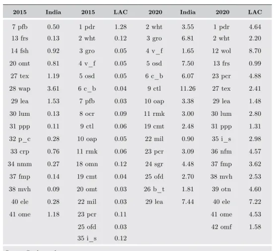
(18) 164. LATIN AMERICAN JOURNAL OF ECONOMICS | V.  N.  (N, ), –. two dif ferent phases (Table 7). Changes in output growth vary across the sectors under dif ferent trade scenarios. Sectoral output growth increased for a few agricultural sectors (plant-based fibers, fishing and forestry) and almost all manufacturing sectors in India due to tarif f reduction in 2015. Meanwhile, at 2020 sectoral output growth is concentrated primarily in agricultural sectors and leather. On the other hand, in Latin America a large number of sectors (agriculture and manufacturing) show positive growth due to tarif f reduction compared to BAU in both scenarios. Some common sectors such as wheat, vegetables, fruit and nuts, processed rice and leather increase output in both economies at 2020. Import tarif f reduction in bilateral trade (India and LAC) is likely to favorably influence the two economies. Here, the sectoral tarif f reduction in India would, it is expected, positively influence the output growth of the same sector in LAC and vice versa. However, as shown in Table 7, one-to-one correspondence does not occur for certain sectors where tarif f cuts are imposed. For example, India’s tarif f reduction on textiles induces textile output expansion in LAC, while for food products LAC does not show gains in 2020. On the other hand, LAC’s reduction of bovine meat tarif fs produces positive output growth of the same sector in India, while this does not occur for electronic equipment. In order to better understand the impacts of freer trade between LAC and India on exports, we turn to tables 5.4 through 5.6.. Export growth The performance of total exports reflects wide variations in growth among the six regions under BAU scenarios (Table 8). India is expected to achieve the highest growth followed by Rest of Asia and LAC countries. On the other hand, the EU shows the lowest export growth under BAU (2015-20). The direction of the percentage change in exports in India and LAC countries under tarif f reduction compared to BAU provides more insight (Table 9)..

(19) 165. K. Mukhopadhyay, P.J. Thomassin, and D. Chakraborty | FREER TRADE IN LAC. Table 7.. Changes in output for selected sectors in India and Latin America in dif ferent trade scenarios compared to BAU (%). 2015. India. 2015. LAC. 2020. India. 2020. LAC. 7 pfb. 0.50. 1 pdr. 1.28. 2 wht. 3.55. 1 pdr. 4.64. 13 frs. 0.13. 2 wht. 0.12. 3 gro. 6.81. 2 wht. 2.20. 14 fsh. 0.92. 3 gro. 0.05. 4 v_f. 1.65. 12 wol. 8.70. 20 omt. 0.81. 4 v_f. 0.05. 5 osd. 7.50. 13 frs. 0.99. 27 tex. 1.19. 5 osd. 0.05. 6 c_b. 6.07. 23 pcr. 4.88. 28 wap. 3.61. 6 c_b. 0.04. 9 ctl. 11.26. 27 tex. 2.41. 29 lea. 1.53. 7 pfb. 0.03. 10 oap. 3.38. 29 lea. 1.48. 30 lum. 0.13. 8 ocr. 0.09. 11 rmk. 3.00. 30 lum. 2.80. 31 ppp. 0.11. 9 ctl. 0.06. 19 cmt. 2.48. 31 ppp. 1.31. 32 p_c. 0.28. 10 oap. 0.05. 22 mil. 0.90. 35 i_s. 2.98. 33 crp. 0.76. 11 rmk. 0.06. 23 pcr. 3.09. 36 nfm. 4.57. 34 nmm. 0.27. 18 omn. 0.12. 24 sgr. 4.48. 37 fmp. 3.62. 37 fmp. 0.14. 19 cmt. 0.04. 25 ofd. 2.70. 38 mvh. 2.53. 38 mvh. 0.09. 20 omt. 0.03. 26 b_t. 1.81. 39 otn. 4.60. 40 ele. 0.28. 22 mil. 0.03. 29 lea. 7.44. 40 ele. 7.22. 41 ome. 1.18. 23 pcr. 0.11. 41 ome. 4.53. 25 ofd. 0.03. 42 omf. 1.58. 35 i_s. 0.12. Source: Study results. Note 1: Only sectors with positive growth are reported here. Note 2: A list of the abbreviations and their meanings can be found in Appendix A.. Table 8.. Export growth in BAU scenario for six regions. Export growth. Rest of OECD. 2010-15. 2015-20. 4.42. 8.98. Rest of Asia. 16.11. 17.58. India. 39.91. 51.11. LAC. 30.43. 11.06. EU_25. 7.58. 3.12. Rest of World. 8.70. 13.95. Source: Study results.

(20) 166. LATIN AMERICAN JOURNAL OF ECONOMICS | V.  N.  (N, ), –. Table 9.. Direction of exports (% change) for India and LAC under dif ferent trade scenarios compared to BAU 2015. 2020. India. LAC. Rest of OECD. -2.18. Rest of Asia. 10.28. India LAC. India. LAC. -1.42. 0.69. 4.08. -1.17. -4.45. 5.46. 6.8 1.78. 6.61 6.25. EU_25. -3.16. -2.78. 13.21. -10.79. Rest of World. -3.57. -1.33. 26.29. -6.47. 3.15. 0.20. 12.05. 2.65. Total Source: Study results.. Trade liberalization strategies are to some extent favorable for India and LAC for both scenarios compared to BAU. India’s exports to LAC are expected to increase by 1.78 and 6.25% respectively under the dif ferent scenarios, whereas for the rest of the regions the percentage change shows a mixed outcome. For LAC countries, exports to India would increase by 6.8 and 6.61% respectively. However, the percentage changes in exports to other regions show a negative impact for all regions in 2015 and a mixed impact for 2020. Under tarif f reduction, India’s exports would benefit more (3.15 and 12.05%, respectively) than LAC (0.20 and 2.65%, respectively). A look at trade diversion resulting from the tarif f reduction between India and LAC reveals that LAC and Indian exports are diverted from other regions and increase between the two economies. A sharp dif ference is observed regarding trade diversion in two scenarios. In 2015 the direction of trade for India and LAC is more diversified. For example, India’s exports to Rest of OECD, Rest of the World and the EU fall while LAC exports are diverted from all regions under study (except India, of course). On the other hand, in 2020 the diversion is concentrated on one region for India (Rest of Asia) and two regions for LAC (the EU and Rest of the World). The 2020 scenario (with tarif f) compared to the 2020 BAU scenario shows an increase of 6.25% in trade, with LAC reflecting trade creation for India, whereas trade creation for LAC is 6.61%. Normally in a bilateral tarif f reduction scenario, both economies benefit but the impact on other regions may or may not be favorable (Mukhopadhyay and Thomassin, 2008)..

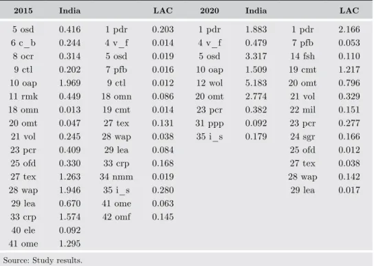
(21) 167. K. Mukhopadhyay, P.J. Thomassin, and D. Chakraborty | FREER TRADE IN LAC. Table 10. Changes in exports for selected sectors in India and Latin America in dif ferent trade scenarios compared to BAU (%) 2015. India. 5 osd 6 c_b 8 ocr 9 ctl 10 oap 11 rmk 18 omn 20 omt 21 vol 23 pcr 25 ofd 27 tex 28 wap 29 lea 33 crp 40 ele 41 ome. 0.416 0.244 0.314 0.202 1.969 0.449 0.013 0.047 0.245 0.409 0.330 1.263 1.946 0.670 1.574 0.092 1.295. 1 pdr 4 v_f 5 osd 7 pfb 9 ctl 18 omn 19 cmt 27 tex 28 wap 29 lea 33 crp 34 nmm 35 i_s 41 ome 42 omf. LAC. 2020. India. 0.203 0.014 0.019 0.016 0.012 0.086 0.014 0.131 0.038 0.084 0.168 0.019 0.280 0.063 0.145. 1 pdr 4 v_f 5 osd 10 oap 12 wol 20 omt 23 pcr 31 ppp 35 i_s. 1.883 0.479 3.317 1.509 5.183 2.774 0.382 0.092 0.179. LAC. 1 pdr 7 pfb 14 fsh 19 cmt 20 omt 21 vol 22 mil 23 pcr 24 sgr 25 ofd 27 tex 28 wap 29 lea. 2.166 0.053 0.110 1.217 0.796 0.329 0.151 0.277 0.166 0.012 0.038 0.142 0.017. Source: Study results. Note 1: Only sectors with positive growth are reported here. Note 2: Appendix A contains a list of the abbreviations and their meanings.. An analysis of the sectoral export growth of India and Latin America due to trade reform shows that it varies in 2015 and 2020 for both economies. In India, sectors favorably af fected in terms of exports are largely agricultural in 2020 and a mixed (agriculture and manufacturing) positive effect is reflected in 2015. For LAC, the sectors that benefit are a combination of agriculture and manufacturing in 2015, while the sectors most affected are processed food and a few industrial sectors (textiles, wearing apparel and leather) at 2020. Tariff reduction has been applied to selected sectors in LAC and India (for details, see Note 1) but the impact is captured across 57 sectors. For example, the tariff reduction on plant-based fibers in India boosts the export of such products from LAC to India, while the reduction in tariffs on meat products in LAC accelerates exports of those products from India to LAC. One interesting feature observed is that the output growth of these two sectors expands (Table 7). The impact of tariff reduction on sectors that LAC and India have in common (textile and leather) varies for both economies..

(22) 168. LATIN AMERICAN JOURNAL OF ECONOMICS | V.  N.  (N, ), –. Welfare impacts It is also of interest to understand the aggregate welfare impacts of trade reforms between LAC and India on both economies as well as the Rest of the World. First we analyze the welfare ef fect of bilateral tarif f cuts between LAC and India. In the global CGE model, each region’s representative agent aims to maximize his/her welfare level. When trade policy is changed, the agent will calculate a change in his/her income level. The change in income level af fects the scale of savings and consumption of each commodity so that the marginal utility of consumption is the same across commodities. In this case, price variables are used in the decision-making process to clear markets in the model. While the welfare level of representative agents in trade agreement member countries (here, India and LAC) would improve, the welfare level of agents in other regions (here, four regions) is likely to decline. Since each region’s welfare function is dif ferent, the impact of trade reforms between India and LAC on the welfare level of the six regions would likely vary. Table 11 summarizes the results of the welfare ef fect (measured as equivalent variation) across the six regions, indicating that gains and losses are not spread evenly. We observed that in the case of tarif f reduction, the welfare of India and Latin America responded differently (US$132.17 million and US$3.81 million for India, US$101.99 million and US$7.03 million for LAC in 2015 and 2020, respectively) under dif ferent scenarios. Rest of OECD, the EU, and Rest of Asia will be the losers in the 2015 tarif f reduction scenario compared to BAU, whereas at 2020 Rest of Asia, the EU and Rest of World will Table 11. Change in welfare in LAC-India under dif ferent trade scenarios (US$ millions) Welfare. 2015. 2020. -83.31. 2.04. Rest of Asia. -90.27. -0.32. India. 132.17. 3.81. LAC. 101.99. 7.03. EU_25. -51.32. -1.32. Rest of World. 49.29. -4.47. Total. 58.86. 6.78. Rest of OECD. Source: Study results..

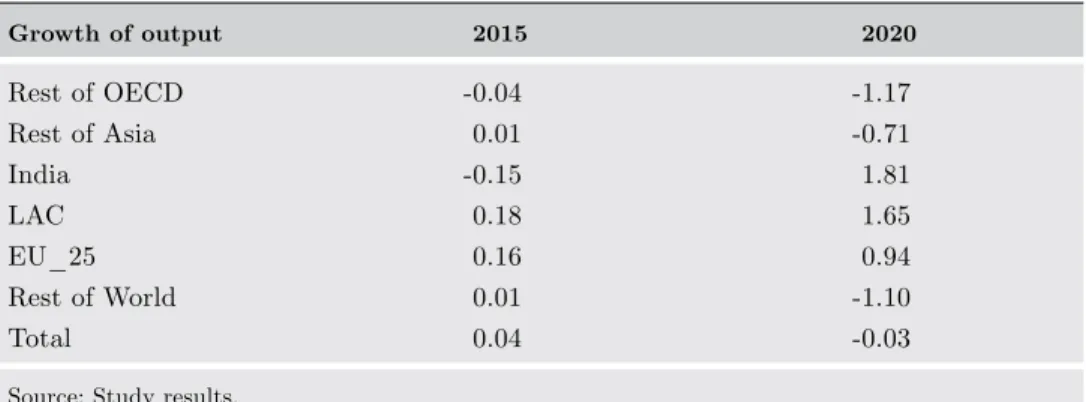
(23) 169. K. Mukhopadhyay, P.J. Thomassin, and D. Chakraborty | FREER TRADE IN LAC. be losers. Global welfare increases by US$58.86 million in 2015 but increases only by US$6.78 million in 2020.. 5.2. LAC and the EU If the ef forts to foster trade liberalization between LAC and the EU materialize, what will be the impact on these two economies in the long run? This section discusses projections for that impact. Changes in selected economic indicators of LAC, the EU and the four other regions resulting from the bilateral tarif f cuts between LAC and the EU are discussed below.. Growth of output As we have seen in the previous section, output growth of the EU and LAC is expected to be 3.78 and 17.27% respectively from 2010 to 2015, while for 2015 to 2020 such growth would be 4.30 and 15.92% respectively. According to the EU-LAC scenario, industrial tariff reduction is imposed on LAC and both industrial and agricultural tarif f reductions are imposed on the EU for the period 2010-20, considering two dif ferent tarif f weights (for details, see Note 2). Both LAC and the EU show positive output growth due to the tarif f reduction, but the other regions perform dif ferently (Table 12). Table 12. EU and Latin America tarif f reduction scenarios compared to BAU Growth of output. Rest of OECD Rest of Asia. 2015. 2020. -0.04. -1.17. 0.01. -0.71. India. -0.15. 1.81. LAC. 0.18. 1.65. EU_25. 0.16. 0.94. Rest of World. 0.01. -1.10. Total. 0.04. -0.03. Source: Study results..

(24) 170. LATIN AMERICAN JOURNAL OF ECONOMICS | V.  N.  (N, ), –. Sectoral performance The percentage change in output growth of selected sectors due to tarif f reduction compared to BAU is presented in Table 13, where positive output growth is shown for tarif f-imposed sectors as well as. Table 13. Changes in output for selected sectors in the EU and Latin America in dif ferent trade scenarios compared to BAU (%) 2015. LAC. 2015. EU. 2020. LAC. 2020. EU. 2 wht. 5.19. 2 wht. 7.66. 3 gro. 10.25. 3 gro. 5.29. 2 wht. 7.44. 2 wht. 11.12. 3 gro. 11.28. 3 gro. 4 v_f. 12.67. 4 v_f. 8.29. 7.47. 4 v_f. 13.71. 4 v_f. 10.85. 5 osd. 7.42. 5 osd. 7.33. 5 osd. 8.94. 5 osd. 8.99. 6 c_b. 9.43. 6 c_b. 4.03. 6 c_b. 10.39. 6 c_b. 7.11 10.82. 8 ocr. 9.71. 8 ocr. 7.64. 8 ocr. 12.00. 8 ocr. 10 oap. 8.20. 10 oap. 4.04. 10 oap. 8.71. 10 oap. 6.10. 18 omn. 1.45. 18 omn. 0.85. 19 cmt. 6.40. 19 cmt. 1.23. 19 cmt. 5.56. 19 cmt. 2.00. 20 omt. 5.31. 20 omt. 2.87. 20 omt. 4.18. 20 omt. 2.14. 21 vol. 2.29. 21 vol. 4.37. 21 vol. 1.99. 21 vol. 3.29. 23 pcr. 8.54. 23 pcr. 9.40. 23 pcr. 11.06. 23 pcr. 7.10. 24 sgr. 3.97. 24 sgr. 2.92. 24 sgr. 3.99. 24 sgr. 2.44. 25 ofd. 3.22. 25 ofd. 0.89. 25 ofd. 3.81. 25 ofd. 1.24. 27 tex. 2.53. 27 tex. 0.46. 27 tex. 2.87. 27 tex. 1.10. 28 wap. 1.10. 29 lea. 2.34. 28 wap. 2.35. 28 wap. 0.38. 29 lea. 1.65. 29 lea. 2.79. 29 lea. 1.91. 36 nfm. 2.02. 30 lum. 0.39. 31 ppp. 0.06. 39 otn. 0.96. 31 ppp. 0.41. 32 p_c. 1.90. 40 ele. 1.07. 32 p_c. 2.91. 33 crp. 0.29. 41 ome. 0.14. 33 crp. 0.49. 34 nmm. 0.59. 40 ele. 1.07. 34nmm. 0.18. 37 fmp. 0.01. 41 ome. 0.14. 38 mvh. 0.04. 41 ome. 0.14. 35 i_s. 0.75. 36 nfm. 1.63. 38 mvh. 0.56. 39 otn. 1.34. 40 ele. 1.05. 41 ome. 0.91. Source: Study results. Note 1: Only sectors with positive growth are reported here. Note 2: Appendix A includes a list of the abbreviations and their meanings..

(25) 171. K. Mukhopadhyay, P.J. Thomassin, and D. Chakraborty | FREER TRADE IN LAC. for other sectors. Highest output growth is observed for vegetables, fruit and nuts, grains nec., crops nec. and sugarcane and sugar beet for both regions during 2010-20. For some sectors, despite the application of tarif f reduction, there is no increase in output growth (for example, forestry) and therefore tarif f reductions in these sectors should be considered carefully by policymakers. On the other hand, some sectors, largely in the agri-food industry, are found to be influenced favorably even without being subject to tarif f reduction under the two scenarios.. Impact on exports The performance of export growth under BAU is recorded in Table 8, indicating wide variations in the export growth of the six regions. It should be noted that exports from LAC and the EU are expected to grow dif ferently under BAU during 2010-20. Exports from LAC would decline sharply from 30.43% in 2010-15 to 11.06% in 2015-20. In the case of the EU, however, the growth rate is expected to decline sharply (from 7.58% in 2010-15 to 3.12% in 2015-20). A look at the direction of the percentage change in exports from LAC and the EU under dif ferent trade scenarios compared to BAU (Table 14) reveals the following: Trade creation is observed in 2015 and 2020 for the EU (0.23 and 0.12% respectively), and LAC (0.79 and 0.66% respectively). The rate of trade creation is expected to decline during this period for Table 14. Direction of % change in exports in LAC and EU scenarios 2015. 2020. EU. LAC. EU. LAC. Rest of OECD. -0.51. -0.19. -0.41. -1.58. Rest of Asia. -0.51. -0.55. -0.37. 0.14. India. -0.16. 1.61. -0.27. 4.97. LAC. 22.26. EU_25 Rest of World Total Source: Study results.. 13.12 9.10. 4.12. -0.29. -0.65. -0.19. 1.92. 0.23. 0.79. 0.12. 0.66.

(26) 172. LATIN AMERICAN JOURNAL OF ECONOMICS | V.  N.  (N, ), –. the two economies. Exports from the EU to LAC are expected to fall significantly from 22.26 to 13.12% from 2015 to 2020. A similar pattern is likely to be observed for exports from LAC to the EU (from 9.12 to 4.12%). It is interesting to note that the percentage change in exports from the EU to LAC (22.26% in 2015) occurs due to exports being withdrawn from other regions of the world and this is expected to continue in 2020, such that trade diversion occurs in both periods. Trade diversion is expected to be dif ferent for LAC, which would likely divert exports from Rest of OECD, Rest of Asia, and Rest of the World in 2015 and only from Rest of OECD in 2020. An analysis of changes in sectoral exports due to tarif f reductions reflects, as shown in Table 15, that the EU gains in the agriculture, processed food and mining sectors at 2020 and manufacturing sectors at 2015. There is a favorable impact for metals nec. and electronic equipment for the EU in 2015, but these sectors do not figure as prominently in 2020. Here, it is important to note that tariff imposition on selected sectors will not always favor those particular sectors’ Table 15. Changes in exports for selected sectors in the EU and Latin America under dif ferent trade scenarios compared to BAU (%) 2020. LAC. EU. 2015. LAC. 3 gro. 0.81. 3 gro. 3.86. 2 wht. 0.91. 5 osd 6 c_b. 2.79. 4 v_f. 4.26. 5 osd. 1.23. 5 osd. 2.19. 6 c_b. EU. 3 gro. 1.45. 0.59. 4 v_f. 3.87. 0.37. 23 pcr. 0.27. 8 ocr. 4.0. 7 pfb. 0.15. 8 ocr. 2.16. 27 tex. 0.38. 10 oap. 1.57. 10 oap. 2.32. 10 oap. 1.62. 28 wap. 0.49. 12 wol. 1.17. 18 omn. 8.04. 12 wol. 1.46. 29 lea. 0.75. 13 frs. 1.81. 20 omt. 3.4. 19 cmt. 1.45. 30 lum. 0.42. 18 omn. 2.3. 22 mil. 2.59. 20 omt. 3.58. 31 ppp. 0.14. 19 cmt. 10.6. 24 sgr. 2.06. 21 vol. 1.25. 34 nmm. 0.18. 31 ppp. 0.16. 25 ofd. 0.07. 23 pcr. 0.66. 35 i_s. 0.14. 32 p_c. 1.87. 26 b_t. 1.43. 24 sgr. 1.47. 36 nfm. 0.25. 36 nfm. 0.04. 31 ppp. 0.01. 27 tex. 0.36. 37 fmp. 0.28. 32 p_c. 1.64. 28 wap. 0.32. 40 ele. 0.12. 34 nmm. 0.19. 33 crp. 2.21. 42 omf. 0.61. Source: Study results. Note 1: Only sectors with positive growth are reported here. Note 2: Appendix A contains a list of the abbreviations and their meanings..

(27) 173. K. Mukhopadhyay, P.J. Thomassin, and D. Chakraborty | FREER TRADE IN LAC. access to the partner’s market. However, indirect impacts may be felt that could stimulate export growth in other sectors, which may be due to direct and indirect interactions among all sectors within a country and across regions. Apart from that, it should be mentioned that there are only 57 sectors classified in GTAP version 7, which is fairly aggregated. In many cases a product part is traded, the impact of which is not reflected in the current classification scheme. This may create dif ficulties in explaining the impact of commodities for manufacturing industries. Further disaggregation of sectors in GTAP would be helpful in capturing the ef fect. The number of sectors af fected in the agriculture group is greater for LAC compared to the EU for both periods. This is expected because the EU would reduce import tarif fs on both agriculture and manufacturing sectors (for details, see Appendix C). LAC is expected to benefit particularly from oilseeds, crops nec., bovine cattle, horse and goat meat products for both periods.. Welfare effect Table 16 presents the welfare gains resulting from the tariff cut between the EU and LAC in 2015 and 2020. Global welfare is expected to reach US$6.086 billion in 2015 and US$2.436 billion in 2020. Welfare gains are observed for the EU, LAC and India under dif ferent trade scenarios, while other regions of the world show a reduction in welfare under LAC-EU tarif f reduction scenarios. Table 16. Change in welfare in LAC-EU under dif ferent scenarios (US$ millions) Welfare. 2015. 2020. Rest of OECD. -1233.30. -1159.56. Rest of Asia. -4359.51. -150.43. India. 1675.12. 85.75. LAC. 8912.06. 628.15. EU_25. 2028.62. 3327.09. Rest of World. -937.01. -294.94. Total. 6085.85. 2436.07. Source: Study results..

(28) 174. 6.. LATIN AMERICAN JOURNAL OF ECONOMICS | V.  N.  (N, ), –. CONCLUSION. This paper makes a modest attempt to forecast the impact of trade reforms between LAC-India on the one hand and LAC-EU on the other in 2020 using a global computable general equilibrium model. A number of simulation exercises relating to alternative trade policies (implementation of import tarif f reductions) were carried out between LAC-India and LAC-EU in 2010, 2015 and 2020 specifically to study the implications of tarif f reduction policies. The findings show that the output of six economies varies under BAU in 2020. The bilateral tarif f reduction scenarios for LAC and India and LAC and the EU reflect that the countries who are parties to the agreement benefit but the impact on other countries is not so favorable. As a result of the tarif f reduction between LAC and India, India’s exports to LAC increase through diversion of exports from other countries and vice versa. Overall, both LAC and India gain more than they lose in exports after tarif f reduction. Tarif f reduction between LAC and the EU broadly indicates trade creation and trade diversion under both scenarios. What emerges from these two experiments (tarif f cuts between LACIndia and LAC-EU) is worth noting for policymakers. LAC will benefit more from trading with India compared to the EU in the long run (2020) while the opposite would likely be true in the short run (2015). In the case of LAC-India trade reform, LAC will divert its trade from the EU to enter the Indian market (Table 5.5) at 2020, while in the case of LAC-EU reform, LAC does not divert its trade from India to capture more of the EU market at 2020 (Table 14). As a result, a welfare loss for the EU is reflected at 2020 (US$-1.32 million) under LAC-India trade reform, while India shows a welfare gain under LAC-EU trade reform. Thus the policy of trade liberalization is likely to be beneficial for LAC and India but not for the EU in the long run. Variation among sectors is observed for outputs and exports for LAC, the EU and India under dif ferent scenarios, such that one-to-one correspondence between the sectors with tarif f reduction and the expected favorable impacts on those sectors’ output and exports is not always apparent from the results. Instead, in some cases there are negative impacts for both the LAC and Indian economies and the same is true for the EU and LAC. It has also been found that sectors not subject to tarif f cuts record positive growth in output and exports. This result, although thought-provoking, may be due to the interdependence of.

(29) K. Mukhopadhyay, P.J. Thomassin, and D. Chakraborty | FREER TRADE IN LAC. 175. sectors within the country and across the dif ferent economies of the world, the functioning of which has been theoretically and empirically simulated by the global computable general equilibrium model used in this study. The welfare impact of bilateral trade reforms is found to be positive for India, LAC and the EU. Our findings show that LAC-EU tarif f reduction appears to be beneficial for both regions in the short run, though not so in the long run. On the other hand, the LAC-India tarif f reduction impact appears to be more beneficial for both economies in the long run than in the short run. This important finding emphasizes the scope and opportunities for south-south cooperation in the long run. In terms of policy, it appears that trade liberalization merits consideration in Latin America and the Caribbean given the long-run benefits, but further investigation is required. One of the limitations of this study is that it considers LAC as a whole, making it dif ficult to identify which LAC countries will gain or lose from expanded trade integration. In addition, the study considers only the uniform application of tarif f reduction across the LAC region, which can lead to overestimates or underestimates in terms of the results in some cases. Most importantly, this study is based on the GTAP framework, which represents direct and indirect interactions among all sectors of the economy and also among dif ferent economies, with precise detailed quantitative results. These are the advantages of most multisector CGE models and not only of GTAP. The main weakness of GTAP is its static nature, which may undermine longhorizon forecasts as is partly reflected in the result..

(30) 176. LATIN AMERICAN JOURNAL OF ECONOMICS | V.  N.  (N, ), –. REFERENCES Armington, P.S (1969), “A theory of demand for products distinguished by place of production, International Monetary Fund Staf f Papers 16: 159-176. Dimaranan. B., ed. (2006), Global Trade, Assistance and Production: The GTAP 6 Database. West Lafayette, IN: Centre for Global Trade Analysis, Purdue University. ECLAC (2009), Economic Survey of Latin America and the Caribbean 2008-2009: Policies for Creating Quality Jobs, Santiago, Chile: United Nations Economic Commission for Latin America and the Caribbean. . (2010-11), Economic Survey of Latin America and the Caribbean 2010-2011, Briefing Paper, Santiago, Chile: United Nations, Economic Commission for Latin America and the Caribbean. . (2010), Latin America and the Caribbean in the World Economy (20092010): A Crisis Generated in the Centre and a Recovery Driven by the Emerging Economies, Santiago, Chile: United Nations, Economic Commission for Latin America and the Caribbean (ECLAC), International Trade and Integration Division. European Commission, Directorate General for Trade (2011), http://ec.europa. eu/trade/creating-opportunities/bilateral-relations/statistics/regions/ European Union MEMO/08/286 (2008), «EU-Latin America Relations on the Eve of the Lima Summit,» Brussels, May 6. European Union MEMO/08/303 (2008), «EU-Latin America/Caribbean Trade in Facts and Figures,» Brussels, May 14. European Union MEMO/10/191 (2010), «The EU, Latin America and the Caribbean (LAC) Strategic Partnership at the eve of the Madrid Summit – Working Together in a Globalised World,» Brussels, May 17. Government of India, Ministry of Commerce and Industry, Department of Commerce, “Focus: LAC (2008), http://commerce.nic.in/flac/flac9.htm Governmen t of India, Ministry of Commerce and Industry, Department of Commerce (2012) «Export-Import Data Bank, TRADESTAT Version 6. Hertel, T.W, ed. (1997), Global Trade Analysis: Modeling and Applications, United Kingdom: Cambridge University Press. Lederman, D., M. Olarreaga, and E. Rubiano (2008), “Trade specialization in Latin America: The impact of China and India,” Review of World Economics, Vol. 144, No. 2: 248-271. Madrid Declaration (2010), VI European Union – Latin America and Caribbean Summit, “Towards a New Stage in the Bi-Regional Partnership: Innovation and Technology for Sustainable Development and Social Inclusion,” Madrid. McDonald, S., S. Robinson, and K. Thierfelder, “Asian Growth and Trade Poles: India, China and East and Southeast Asia,”. Presented at the 10th Annual Conference on Global Economic Analysis, June 2007, Purdue University. https://www.gtap.agecon.purdue.edu/resources/res_display. asp?RecordID=2355.

(31) K. Mukhopadhyay, P.J. Thomassin, and D. Chakraborty | FREER TRADE IN LAC. 177. Moreira, M.M. (2010), “India: Latin America’s Next Big Thing,” Special Report on Integration and Trade, Washington, D.C.: Inter-American Development Bank. Mukhopadhyay, K. and P.J. Thomassin (2008), “Impact Of Trade Liberalisation on the Environment – Illustrations from East Asia,” GTAP Resource #2634, West Lafayette, IN: Purdue University. . (2010), Economic and Environmental Impact of Free Trade in East and South East Asia, The Netherlands: Springer. Narayanan, B.G. and T.L. Walmsley (2008), “Global Trade, Assistance, and Production: The GTAP 7 Data Base”, West Lafayette, IN: Center for Global Trade Analysis, Purdue University. Ram, M. (1971), “India’s trade prospects in Latin America,” Economic and Political Weekly, Vol. 6, No.47: 2347-2349. Rojas-Romagosa, H. and L. Rivera (2007), “Economic implications of an association agreement between the European Union and Central America,” Institute for International and Development Economics Discussion Paper. United Nations Secretariat, Department of Economic and Social Affairs, Population Division (2006), World Population Prospects: The 2006 Revision Population Database, Population and Economically Active Population (Version 5). World Development Indicators, Real Historical and Projected Gross Domestic Product (GDP) and Growth Rates of GDP for Baseline Countries /Regions 2000-2017, 2007, Washington, D.C.: World Bank..

(32) 178. LATIN AMERICAN JOURNAL OF ECONOMICS | V.  N.  (N, ), –. APPENDIX A Table A1. Sectoral classification in GTAP Version 7 pdr Paddy rice. wht Wheat. gro. Cereal grains nec.. osd. Oil seeds. v_f Vegetables, fruit, nuts. pfb. Plant-based fibers. ocr. ctl. Cattle, sheep, goats, horses. oap Animal products nec.. c_b Sugar cane, sugar beet Crops nec.. rmk Raw milk. wol Wool, silk-worm cocoons. frs. Forestry. fsh. Fishing. coa. Coal. oil. Oil. gas. Gas. omn Minerals nec.. cmt Meat: cattle, sheep, goat, horse. omt Meat products nec.. vol. Vegetable oils and fats. mil. Dairy products. pcr. Processed rice. sgr. Sugar. ofd. Food products nec.. b_t Beverages and tobacco products. tex. Textiles. wap Wearing apparel. lea. Leather products. lum Wood products. ppp Paper products, publishing. p_c Petroleum, coal products. crp. Chemical, rubber, plastic products. nmm Mineral products nec.. i_s. Ferrous metals. nfm Metals nec.. fmp Metal products. mvh Motor vehicles and parts. otn. ele. Transport equipment nec.. Electronic equipment. ome Machinery and equipment nec.. omf Manufactures nec.. ely. gdt. Gas manufacture, distribution. wtr Water. Electricity. cns. Construction. trd. otp. Transport nec.. wtp Sea transport. atp. Air transport. cmn Communication. ofi. Financial services nec.. isr. Insurance. obs. Business services nec.. ros. Recreation and other services. osg. PubAdmin/Defence/Health/Education. Trade. dwe Dwellings Source: Narayanan and Walmsley (2008)..

(33) K. Mukhopadhyay, P.J. Thomassin, and D. Chakraborty | FREER TRADE IN LAC. 179. APPENDIX B Table B1. Trade agreements in force Customs unions Andean Community Caribbean Community (CARICOM) Central American Common Market (CACM) MERCOSUR Free trade agreements Partner countries. Date Date of entry of signature into force. Bolivia - MERCOSUR. 17 Dec 1996. 28 Feb 1997. Bolivia - Mexico. 17 May 2010. 07 Jun 2010. Canada - Chile. 05 Dec 1996. 05 Jul 1997. Canada - Colombia. 21 Nov 2008. 15 Aug 2011. Canada - Costa Rica. 23 Apr 2001. 01 Nov 2002. Canada - EFTA. 26 Jan 2008. 01 Jul 2009. Canada - Israel. 31 Jul 1996. 01 Jan 1997. Canada - Peru. 29 May 2008. 01 Aug 2009. CARICOM - Costa Rica. 09 Mar 2004. CARICOM - Dominican Republic. 22 Aug 1998. CARIFORUM - European Union. 15 Oct 2008. Central America - Chile. 18 Oct 1999. Central America - Dominican Republic. 16 Apr 1998. Central America - Panama. 06 Mar 2002. 29 Dec 2008. Chile - Australia. 30 Jul 2008. Chile - China. 18 Nov 2005. 06 Mar 2009 01 Oct 2006. Chile - Colombia. 27 Nov 2006. 08 May 2009. Chile - EFTA. 26 Jun 2003. 01 Dec 2004. Chile - EU. 18 Nov 2002. 01 Feb 2003. Chile - Japan. 27 Mar 2007. 03 Sep 2007. Chile - Korea. 15 Feb 2003. 01 Apr 2004. Chile - MERCOSUR. 25 Jun 1996. 01 Oct 1996. Chile - Mexico. 17 Apr 1998. 01 Aug 1999. Chile - New Zealand, Singapore and Brunei Darussalam (P4). 18 Jul 2005. Chile - Panama. 27 Jun 2006. 07 Mar 2008. Chile - Peru. 22 Aug 2006. 01 Mar 2009. Chile - Turkey. 14 Jul 2009. 01 Mar 2011. Chile - United States. 06 Jun 2003. 01 Jan 2004.

(34) 180. LATIN AMERICAN JOURNAL OF ECONOMICS | V.  N.  (N, ), –. Table B1. (continued) Partner countries. Date Date of entry of signature into force. Colombia - European Free Trade Association (EFTA). 25 Nov 2011. Colombia - Mexico. 13 Jun 1994. Colombia - Northern Triangle. 09 Aug 2007. Costa Rica - China. 08 Apr 2010. 01 Aug 2011. Costa Rica - Mexico. 05 Apr 1994. 01 Jan 1995. DR-CAFTA (Central America - Dominican Republic - United States). 05 Aug 2004. El Salvador - Taiwan. 07 May 2007. Guatemala - Taiwan. 22 Sep 2005. Honduras - Taiwan. 07 May 2007. 01 Jul 2011. 01 Jul 2005. MERCOSUR - Israel. 18 Dec 2007. MERCOSUR - Peru. 30 Nov 2005. Mexico - EFTA. 27 Nov 2000. 01 Jul 2001. Mexico - EU. 08 Dec 1997. 01 Jul 2000. Mexico - Israel. 10 Apr 2000. 01 Jul 2000. Mexico - Japan. 17 Sep 2004. 01 Apr 2005. Mexico - Nicaragua. 18 Dec 1997. 01 Jul 1998. Mexico - Northern Triangle. 29 Jun 2000. Mexico - Peru. 06 Apr 2011. Mexico - Uruguay. 15 Nov 2003. 15 Jul 2004. NAFTA (Canada - Mexico - United States). 17 Dec 1992. 01 Jan 1994. Nicaragua - Taiwan. 16 Jun 2006. 01 Jan 2008. Panama - Singapore. 01 Mar 2006. 24 Jul 2006. Panama - Taiwan. 21 Aug 2003. 01 Jan 2004. Peru - China. 28 Apr 2009. 01 Mar 2010. Peru - European Free Trade Association (EFTA). 14 Jul 2011. 01 Jul 2011. Peru - Japan. 31 May 2011. 01 Mar 2012. Peru - Singapore. 29 May 2008. 01 Aug 2009. Peru - South Korea. 14 Nov 2010. 01 Aug 2011. Peru - Thailand. 31 Dec 2011. 01 Feb 2012. Peru - United States. 12 Apr 2006. 01 Feb 2009. United States - Australia. 18 May 2004. 01 Jan 2005. United States - Bahrain. 14 Sep 2004. 01 Jan 2006. United States - Israel. 22 Apr 1985. 01 Sep 1985. United States - Jordan. 24 Oct 2000. 17 Dec 2001. United States - Morocco. 15 Jun 2004. 01 Jan 2006. United States - Oman. 19 Jan 2006. 01 Jan 2009. United States - Singapore. 06 May 2003. 01 Jan 2004. United States - South Korea. 30 Jun 2007. 15 Mar 2012.

(35) K. Mukhopadhyay, P.J. Thomassin, and D. Chakraborty | FREER TRADE IN LAC. 181. Table B1. (continued) Framework agreements Partner countries MERCOSUR - India. Date Date of entry of signature into force 25 Jan 2004. 01 Jun 2009. MERCOSUR - Mexico (ACE54) - framework agreement. 05 Jul 2002. 05 Jan 2006. MERCOSUR - Mexico (ACE55) - auto sector agreement. 27 Sep 2002. Partial preferential agreements Partner countries Andean countries (Colombia, Ecuador, Venezuela) - MERCOSUR. Date Date of entry of signature into force 18 Oct 2004. Argentina - Brazil (ACE No 14). 20 Dec 1990. 20 Dec 1990. Argentina - Chile (AAP.CE No 16). 02 Aug 1991. 02 Aug 1991. Argentina - Mexico (ACE No 6). 28 Nov 1993. 01 Jan 1987. Argentina - Paraguay (ACE No13). 06 Nov 1992. 06 Nov 1992. Argentina - Uruguay (AAP.CE No 57). 31 Mar 2003. 01 May 2003. Bolivia - Chile (AAP.CE No 22). 06 Apr 1993. 06 Apr 1993. Brazil - Guyana (AAP.CE No 38). 27 Jun 2001. 31 May 2004. Brazil - Mexico (AAP.CE No 53). 03 July 2002. 02 May 2003. Brazil - Uruguay. 30 Sep 1986. 01 Oct 1986. CARICOM - Colombia. 24 July 1994. 01 Jan 1995. CARICOM - Venezuela. 13 Oct 1992. 01 Jan 1993. Chile - Ecuador (AAP.CE No 32). 20 Dec 1994. 20 Dec 1994. Chile - Venezuela (AAP.CE No 23). 02 Apr 1993. 02 Apr 1993. Colombia - Costa Rica (AAP.A25TM No 7). 02 Mar 1984. Colombia - Honduras. 30 May 198. Colombia - Nicaragua (AAP.AT25TM Nº 6). 02 Mar 1984. Colombia - Panama (AAP.AT25TM Nº 29). 09 July 1993. 18 Jan 1995. Colombia - Venezuela. 28 Nov 2011. 16 Apr 2012. Costa Rica - Venezuela (AAP.A25TM No 26). 21 Mar 1986. Dominican Republic - Panama. 17 July 1985. Ecuador - Paraguay (AAP.CE No 30). 15 Sep 1994. Ecuador - Uruguay (AAP.CE No 28). 01 May 1994. El Salvador - Venezuela (AAP.A25TM No 27). 10 Mar 1986. Guatemala - Venezuela (ACE No 23). 10 Oct 1985. 8 June 1987 01 Apr 2005. Guyana - Venezuela (AAP.A25TM No 22). 27 Oct 1990. Honduras - Panama. 08 Nov 1973. Honduras - Venezuela (AAP.A25TM No 16). 20 Feb 1986. Mexico - Panama (AAP.A25TM No 14). 22 May 1985. 24 Apr 1986. Mexico - Peru (ACE No 8). 29 Jan 1995. 25 Mar 1987. Nicaragua - Panama. 26 July 1973. 18 Jan 1974. Nicaragua -Venezuela (AAP.A25 TM No 25). 15 Aug 1986. Trinidad and Tobago - Venezuela (AAP.A25TM No 20). 04 Aug 1989. Source: http://www.sice.oas.org/agreements_e.asp. 28 June 1991.

(36) 182. LATIN AMERICAN JOURNAL OF ECONOMICS | V.  N.  (N, ), –. APPENDIX C Specific commodities have been identified for tarif f reduction on the basis of a recent proposed agreement between India and Latin American countries. Table C1. Tarif f reduction on commodities in LAC and India LAC. India. Cattle, sheep, goats, horses. Plant based fiber. Forestry. Food products. Minerals nec.. Textiles. Meat: cattle, sheep, goats, horse. Wearing apparel. Meat products nec.. Leather products. Textile. Chemical, rubber, plastic products. Wearing apparel. Electronic equipment. Leather products. Machinery and equipment nec.. Wood products Paper products, publishing Chemical, rubber, plastic products Mineral products nec. Ferrous metals Electronic equipment Machinery and equipment nec. Manufactures nec. Source: Focus: LAC (2008)..