Following up the First Detection of Gravitational Waves with Numerical Relativity Simulations

Texto completo

(1)Following up the First Detection of Gravitational Waves with Numerical Relativity Simulations Alfred Castro Ginard. Master’s Thesis. Master’s degree in Physics (With a speciality/Itinerary in Astrophysics and Relativity) at the UNIVERSITAT DE LES ILLES BALEARS. Academic year 2015-16. Date: September, 2016. UIB Master’s Thesis Supervisor Dr. Sascha Husa. Author signature ________________. Supervisor signature _____.

(2) ii.

(3) Abstract. The first detection of a gravitational wave signal occurred on September 14 2015, when the two LIGO detectors in Hanford and Livingston registered a consistent signal with a statistical significance of more than 5 relative to the background noise. In order to identify the source of gravitational wave signals, they need to be compared with theoretical predictions. In the case of the first detection, the signal was found consistent with the prediction of general relativity for the waves produced by the last orbits and coalescence of two black holes with initial masses 36M and 29M , leading to a final black hole mass of 62M with 3.0M c2 radiated in gravitational waves. The modern theory of gravitation is Einstein’s theory of general relativity, and modelling possible signals with solutions of the Einstein equations is a key goal for gravitational wave physics. Perturbative methods, as have been used for the indirect discovery by Hulse, Taylor, and Weisberg [1, 2] of gravitational wave emission from the binary pulsar PSR B1913+16 in 1974, break down in the strong field regime of general relativity, and to model the merger of black holes, the methods of numerical relativity to solve the Einstein equations without physical approximations need to be used. In this thesis a precessing waveform compatible with the first detection event, GW150914, is constructed by numerical solution of the Einstein field equations as a system of coupled nonlinear partial di↵erential equations, and compared with the data recorded by the LIGO detectors. Perturbative methods are used to compute initial parameters for the black holes, and to construct a complete waveform by matching the numerical and perturbative solutions. Physical properties of the solution are computed and discussed, such as the final spin, final mass, recoil velocity and energy distribution for di↵erent spherical harmonic modes of the wave signal. iii.

(4) The Einstein evolution equations can be considered a nonlinear system of wave equations, and the numerical solution of the linear wave equation is discussed to introduce the numerical finite di↵erence methods used.. iv.

(5) Acknowledgements. I would like to thank to my thesis advisor, Dr. Sascha Husa, for giving me the opportunity to work with him, the guidance and patience during these years. I would also like to thank to Xisco Jiménez Forteza, for his helpful talks and for the time we spent working together. Also thank to my office partner, Pep Covas, for his useful contributions during this year. Also, thank to all the LIGO@UIB group, specially to Dr. Alicia Sintes and Dr. David Keitel for their valuable suggestions. Finally, thank to the Institute of Applied Computing with Community Code (IAC3 ) for giving me their introduction to research scholarship.. v.

(6) vi.

(7) To my parents. vii.

(8) viii.

(9) Contents. 1 Introduction. 1. 2 Black Holes, Binaries and Gravitational Waves. 5. 2.1. Schwarzschild Geometry . . . . . . . . . . . . . . . . . . . . . . . . . . . .. 6. 2.2. Kerr Geometry . . . . . . . . . . . . . . . . . . . . . . . . . . . . . . . . .. 6. 2.3. Horizons . . . . . . . . . . . . . . . . . . . . . . . . . . . . . . . . . . . . .. 7. 2.3.1. Trapped Surfaces and Apparent Horizons . . . . . . . . . . . . . . .. 7. 2.4. Black Hole Binaries . . . . . . . . . . . . . . . . . . . . . . . . . . . . . . .. 8. 2.5. Gravitational Waves . . . . . . . . . . . . . . . . . . . . . . . . . . . . . .. 9. 3 E↵ective One-Body approach. 11. 3.1. Orbital Hamiltonian . . . . . . . . . . . . . . . . . . . . . . . . . . . . . .. 11. 3.2. Spin contribution . . . . . . . . . . . . . . . . . . . . . . . . . . . . . . . .. 12. 3.3. Equations of motion and conserved quantities . . . . . . . . . . . . . . . .. 13. 3.4. Radiation Reaction . . . . . . . . . . . . . . . . . . . . . . . . . . . . . . .. 14. 4 Mathematical Procedure 4.1 4.2. 4.3. 17. Initial Value Problem . . . . . . . . . . . . . . . . . . . . . . . . . . . . . .. 17. 4.1.1. Well-posedness . . . . . . . . . . . . . . . . . . . . . . . . . . . . .. 18. The 3+1 Decomposition . . . . . . . . . . . . . . . . . . . . . . . . . . . .. 18. 4.2.1. Extrinsic Curvature . . . . . . . . . . . . . . . . . . . . . . . . . . .. 21. 4.2.2. Decomposition of the Riemann tensor . . . . . . . . . . . . . . . . .. 22. The York-ADM equations . . . . . . . . . . . . . . . . . . . . . . . . . . .. 24. ix.

(10) 4.4. The BSSN equations . . . . . . . . . . . . . . . . . . . . . . . . . . . . . .. 5 Numerical Procedure. 24 29. 5.1. Initial Data . . . . . . . . . . . . . . . . . . . . . . . . . . . . . . . . . . .. 29. 5.2. Evolution . . . . . . . . . . . . . . . . . . . . . . . . . . . . . . . . . . . .. 31. 5.2.1. Conformal factor . . . . . . . . . . . . . . . . . . . . . . . . . . . .. 32. 5.2.2. Gauge conditions . . . . . . . . . . . . . . . . . . . . . . . . . . . .. 33. Numerical Method . . . . . . . . . . . . . . . . . . . . . . . . . . . . . . .. 33. 5.3.1. Evolution Method . . . . . . . . . . . . . . . . . . . . . . . . . . . .. 34. 5.3.2. Adaptive Mesh Refinement . . . . . . . . . . . . . . . . . . . . . . .. 34. 5.3.3. Extraction quantities . . . . . . . . . . . . . . . . . . . . . . . . . .. 35. Wave equation as a Toy Model for Hyperbolic Equations . . . . . . . . . .. 39. 5.3. 5.4. 6 Numerical Simulations of a Precessing q = 1.2 Black Hole Binary 6.1. 45. Runs Configuration . . . . . . . . . . . . . . . . . . . . . . . . . . . . . . .. 46. 6.1.1. Convergence Test . . . . . . . . . . . . . . . . . . . . . . . . . . . .. 49. 6.1.2. Richardson Extrapolation . . . . . . . . . . . . . . . . . . . . . . .. 51. 6.2. Precession . . . . . . . . . . . . . . . . . . . . . . . . . . . . . . . . . . . .. 52. 6.3. Results . . . . . . . . . . . . . . . . . . . . . . . . . . . . . . . . . . . . . .. 53. 6.3.1. Final Mass and final spin . . . . . . . . . . . . . . . . . . . . . . . .. 55. 6.3.2. Final Recoil Velocity . . . . . . . . . . . . . . . . . . . . . . . . . .. 56. Waveform . . . . . . . . . . . . . . . . . . . . . . . . . . . . . . . . . . . .. 57. 6.4.1. . . . . . . . . . . . . . . . . . . . . . . . . . . . . . . . . . . . .. 58. Fixed Frequency Integration (FFI) Method . . . . . . . . . . . . . .. 59. 6.4. 6.4.2. 4. 7 The Detected Gravitational Wave Signal. 63. 7.1. Spin Weighted Spherical Harmonics . . . . . . . . . . . . . . . . . . . . . .. 64. 7.2. Gravitational Wave Signal in the Detector Frame . . . . . . . . . . . . . .. 64. 7.2.1. Sky Location . . . . . . . . . . . . . . . . . . . . . . . . . . . . . .. 66. 7.2.2. The Detected Wave . . . . . . . . . . . . . . . . . . . . . . . . . . .. 68. 7.3. GW150914 Data Analysis . . . . . . . . . . . . . . . . . . . . . . . . . . .. 69. 7.4. Comparison to Real Data . . . . . . . . . . . . . . . . . . . . . . . . . . .. 71. 8 Conclusions. 75 x.

(11) Bibliography. 77. xi.

(12) xii. Alfred Castro.

(13) Chapter. 1. Introduction Albert Einstein’s theory of General Relativity (GR) [3] provides a di↵erent description of gravitation than Newtonian gravity, mathematically and conceptually. It starts from the fact that acceleration of the objects is not due to a force but due to the geometry of the space-time itself. In Newtonian mechanics, the force of gravity can be described in terms on its gravitational potential , that comes from a continuous mass distribution ⇢, defined using the Laplace operator as, = 4⇡G⇢.. (1.1). In GR, gravity is not a force but geometry, the gravitational potential. is replaced by the. metric tensor gab , which contains the information of the geometric structure of the spacetime: and the mass distribution ⇢ is now replaced by the distribution of matter and energy, the stress-energy tensor Tab . The sources of the curvature and the space-time’s geometry can be related with the Einstein field equations, and, equation (1.1) can be replaced by, Gab =. 8⇡G Tab , c4. where the Einstein tensor Gab , defined as Gab = Rab. (1.2) 1 Rgab , 2. depends on the metric. tensor, so it describes the geometry of the space-time. The indices {a, b} goes from zero to three denoting the di↵erent temporal (0) and spatial (1-3) dimensions. So, the problem. of modelling the evolution of a black hole binary consists in solving the Einstein vacuum equations (Rab = 0). On one hand, in Newtonian gravity, the interaction of two point masses represents the simplest non-trivial problem, it describes a wide range of physical situations, and, in 1.

(14) addition, it can be solved analytically. On the other hand, GR presents a more complicate and completely new theory. In General Relativity, as it is known, the two body problem loses energy which is radiated as gravitational radiation that propagates away from the source as waves at the speed of light. Thus, the two body problem in GR is unstable, and it will result in the shrink of the orbit that will lead to the collision of the two objects. Gravitational waves are generated by accelerated masses, and, the most massive and accelerated the objects are, the most energetic gravitational waves they will emit. To generate such gravitational waves, the two objects need to be massive objects orbiting at very close separations. So, now, the most compact objects are not point particles anymore but black holes. The study of the two body problem has now become to the study of a black hole binary. The two body problem now represents a huge challenge, from considering an ordinary di↵erential equation (ODE) in Newtonian Gravity and find its solution; to numerically solve, in GR, a set of ten coupled, non-linear second order partial di↵erential equations (PDE’s). The field of Numerical Relativity is dedicated to the construction of black hole spacetimes by numerically integrating the Einstein’s equations (1.2). The first attempt of solving them, for two black holes, was done by Hahn and Lindquist in 1964 [4], but at the time, although they knew a procedure for the numerical integration, due to insufficient computational resources, inadequate gauge conditions and the lack of a well-posed formulation, they could only evolve their data for a short time. Significant breakthrough was made at 2005 when the first numerical simulations that include the merger and ringdown phases were carried out by Pretorius [5]. Since then, simulations of black hole binaries in the field of Numerical Relativity have given a better insight into the dynamics of binary black hole coalescence. The motivation in the e↵ort of the Numerical Relativity in modelling gravitational wave sources comes from the construction of gravitational wave detectors such as LIGO [6], VIRGO [7] or GEO600 [8]. Waveform catalogues, a library that contains waveforms coming from di↵erent black hole configurations which patterns are searched in the real data, have helped gravitational waves data analysis teams to report the first direct detection of a gravitational wave, GW150914 [9], by the LIGO Scientific Collaboration on September 14, 2015. However, Numerical Relativity is not the only field dedicated to the construction of waveform templates, the signal in the sensitivity band of the detector covers many 2. Alfred Castro.

(15) more orbits than those modeled by Numerical Relativity simulations. Those orbits can be modeled by analytical Post-Newtonian methods, or using e↵ective one-body models because the evolution in the early inspiral stage is adiabatic. Then, the waveform is constructed by stitching together analytical waveforms with numerical ones. This thesis will cover the process of the construction of a precessing waveform model, whose parameters are consistent with GW150914 [10]. Some basic aspects of black holes and gravitational waves needed in this thesis will be covered in Chapter 2. An analytical approach to the first inspiral phase of the binary evolution is given in Chapter 3. A mathematical description of how to get the Einstein field equations in the 3 + 1 form will be explained in Chapter 4. The numerical code used to evolve the black hole binary is described in Chapter 5. Chapter 6 goes through the numerical simulation of the binary black hole merger and it’s results. And finally, a comparison of the waveform constructed and the real data recorded by the detectors is performed in Chapter 7.. Alfred Castro. 3.

(16) 4. Alfred Castro.

(17) Chapter. 2. Black Holes, Binaries and Gravitational Waves We can see the light coming out from a star like our Sun because the speed of light is higher than the escape velocity of the star, given by,. ve =. r. 2GM , R. (2.1). where we see how compact is the star in the relation between its mass and radius M/R. If we invert the problem and see what size the star should have, so that the light can not escape, in the case of our Sun, it would be a radius of about 3km, computed by just inverting equation (2.1), R =. 2GM . c2. When one considers the time evolution of the given star, it will eventually run out of nuclear fuel, consequently, the star will not be able to maintain the equilibrium; so, the star will undergo gravitational collapse. Nevertheless, because of the contraction, the star may change its equation of state, leading to a new equilibrium state. These new equilibrium states can be supported by Fermi pressure of the electrons (white dwarfs) or the neutrons (neutron stars). But when we solve the Tolman-Oppenheimer-Volko↵ (TOV) equations, we see that for a given equation of state there is a maximum mass for the star to be in equilibrium. Because that mass is so large, the Newtonian equation (2.1) gives us velocities higher than the speed of light. To solve that problem, we need to approach the situation from the point of view of the General Relativity. 5.

(18) 2.1. Schwarzschild Geometry. When a spherically symmetric star has collapsed, the whole space-time can be described with the Schwarzschild geometry, which is the most general vacuum solution of the Einstein field equations. The Schwarzschild geometry [11] is an exact solution to the Einstein field equations (1.2) found shortly after their publication by Karl Schwarzschild. The form of the metric is 2. ds =. ✓. 1. 2M r. ◆. 2. ✓. dt + 1. 2M r. ◆. 1. dr2 + r2 (d✓2 + sin2 (✓)d'2 ),. (2.2). note the use of geometric units (G = c = 1) that will be used from now on. At r = 0 and r = 2M the metric coefficients gtt and grr become zero or infinite, but because metric coefficients are coordinate dependent, these singularities could be an e↵ect of the choice of the coordinates, or it could be real singularities in the space-time. To distinguish between both possibilities one have to find a scalar quantity, which is coordinate independent, such as the Riemann Scalar Rabcd Rabcd and see whether it behaves singular or not. For the Schwarzschild metric (2.2), one can see, Rabcd Rabcd =. 48M 2 , r6. (2.3). that r = 0 represents a true singularity. However, the feature that defines a black hole is not its singularity at r = 0 but at r = 2M , where the event horizon forms. The event horizon is null hypersurface which is a boundary in the space-time within which the gravitational attraction is so strong than not even light can escape from it. The description above is for a Schwarzschild black hole, that thanks to the Birkho↵ theorem we know this is the only solution for the space-time outside a spherical, non-rotating, gravitating body that would result from an spherical gravitational collapse. But not only this kind of collapse leads to the formation of a black hole. Nevertheless, the basic picture of the collapse when no spherical simplifications can be applied would remain the same and a black hole would form.. 2.2. Kerr Geometry. One can find a more general family of solutions of (1.2) that leads to the existence of black holes. The no-hair theorem [12] states that all black hole solutions can be described in 6. Alfred Castro.

(19) terms of three parameters: mass (M ), angular momentum (J) and charge (Q). Given that most of the astrophysical objects are neutral (Q = 0), a solution in terms of {M, J} is given by the Kerr metric, that describes the geometry around a rotating black hole, it can be written as, 2. ds =. ✓. 1. 2M r ⇢2. ◆. dt2. 4M ar sin2 (✓) ⇢2 2 2 2 sin2 (✓) dtd'+ dr +⇢ d✓ + (r2 + a2 )2 2 2 ⇢ ⇢. where ⇢2 = r2 + a2 cos2 (✓); and. a2. sin2 (✓) d'2 , (2.4). = r2. 2M r + a2 ; and the Kerr parameter a is defined. by a = J/M . In this metric, we find again singular points when ⇢ = 0 and. = 0. If we analyse. these points analogously to the Shcwarzschild case, the evaluation of the Riemann scalar Rabcd Rabcd shows that ⇢ = 0 is a true singularity, just as r = 0 in the Schwarzschild geometry. Thus, the singularity at. = 0 is a coordinate singularity and, analogous to the. Schwarzschild case, indeed turns out to be the event horizon.. 2.3. Horizons. So far we have just mentioned the event horizon, a region of the space-time that encloses a singularity, and where not even light can escape from it. But from the definition, the event horizon is about the ultimate fate of the observer, it can only be determined if the maximal time development is known. However, it would be useful to describe a similar region but locally in time, so one won’t have to wait till the end of time to locate the horizon. That is the notion of a trapped surface and the apparent horizon.. 2.3.1. Trapped Surfaces and Apparent Horizons. Imagine a sphere in a spatial slice of the space-time ⌃ of constant time coordinate. If we send photons from the sphere surface (S), a light cone will be formed as the photons propagates away from the surface at later times. If the spherical surface encloses a singularity the curvature of the space-time around may be so strong that eventually the path of the outgoing photon may also bend. Alfred Castro. 7.

(20) Figure 2.1: Notion of untrapped (a) and trapped surfaces (b). k. and k + are the null-vectors. associated to the ingoing and outgoing front. Source: https://inspirehep.net/record/1279001/plots. When the rate of change of the area generated by the outgoing front is negative, then we have a trapped surface. The notion of an apparent horizon in derived from the trapped surface: the boundary of the regions of trapped surfaces. So, we define the marginally outer trapped surface (MOTS), represented by the outgoing photon front, when the rate of change of the area generated by the outgoing front becomes zero. And we identify the MOTS as the apparent horizon which is defined at every spatial hypersurface ⌃. Therefore, black holes can be defined by its apparent horizon instead of its event horizon. This is an essential component of binary black hole evolution codes.. 2.4. Black Hole Binaries. The most promising sources of gravitational waves are two black holes orbiting each other forming a bound system. As already mentioned, the two-body problem in GR is not stable, the binary radiates away energy and momentum in the form of gravitational waves resulting in the decay of the orbits until both black holes merge together. The evolution of a black hole binary goes through three di↵erent processes as each black hole moves towards the other. A first, extended phase where the radiation of energy makes the binary adiabatically evolve to smaller separations which is called inspiral. The merger, where the gravitational wave emission is no longer adiabatic and both black holes plunge together and merge. And the last stage, when a single Kerr black hole is formed which is called ringdown. 8. Alfred Castro.

(21) During the inspiral stage, when the two black holes are far enough to be modulated by the Post-Newtonian approximation, gravitational wave emission will remove energy from the binary causing the decrease of the separation of the black holes. At this stage, an analytical approach to the radiated power and thus, to the evolution of the binary separation and to the amplitude of the gravitational waves emitted can be performed using the Post-Newtonian expansion. At the leading order, this energy loss can be modeled by the quadrupole formula as dE = dt where Qij =. R. ⇢(xi xj. ij r. 2. ✓ ◆2 G X d3 Qij , 5c5 i,j dt3. (2.5). /3)d3 x is the mass quadrupole moment.. At the ringdown stage, the remnant black hole can be described as a perturbed Kerr black hole. It has been realized that perturbed black holes have quasi-normal modes of vibration, which are the formal solutions of the linearized di↵erential equations of the General Relativity with complex frequency; and the gravitational waves emitted from the merger can be described as a superposition of these quasi-normal modes, and computed using perturbative techniques [13, 14]. It is during the merger, where the need of computational resources appear. The accurate modelling of this stage is done via Numerical Relativity simulations.. 2.5. Gravitational Waves. Another exciting prediction of the General Relativity is the existence of gravitational waves. They are perturbations of the space-time propagating away from the source as waves at the speed of light, generated by non-spherical or nonuniform mass in motion. Gravitational Waves carry energy as gravitational radiation. Even Gravitational Waves can transport large amounts of energy, they interact very weakly with matter, that is the reason why they are so difficult to detect but at the same time this fact allow them to travel storing the information of the source una↵ected. One can see this weakness in (2.5) with the dependence of the constants G and c, and also comparing the gravitational radiation to the electromagnetic radiation, which its leading order is the dipole instead of the quadrupole moment. The first indirect detection of Gravitational Waves was the observation of the orbital decay of the Hulse-Taylor binary system [1], the energy loss through the emission of graviAlfred Castro. 9.

(22) tational radiation is consistent with the prediction of General Relativity. Since then, many e↵orts have been made to directly detect Gravitational Waves. Ground-based interferometric detectors such as LIGO [6], VIRGO [7], GEO600 [8] have been built resulting in the first direct detection of Gravitational Waves emitted in a binary black hole coalescence [9]. Gravitational waves are detected via interferometric techniques measuring the relative change in the detector’s arms. L/L of length L, see Chapter 7.. Accurate numerical simulations of black hole binaries allow the creation of waveforms catalogues, so one can compare to the real data recorded by the detectors and identify the better gravitational wave model that best represents the data. In further chapters, the waveform emitted by the merger will be constructed via full numerical Relativity. Nevertheless, we can see with simple arguments why it should be a binary black hole [15]. Those arguments are: (i) the frequency and amplitude of the gravitational wave are increasing, this suggest that it should come from the orbital motion of a binary; and (ii) the maximum frequency at which the gravitational radiation is observed tells us how close the orbiting objects should be, only black holes can reach such a small separation.. 10. Alfred Castro.

(23) Chapter. 3. E↵ective One-Body approach In the last moments of a binary black hole coalescence, the Einstein field equations have to be solved via full Numerical Relativity (NR). However, there is no need to solve those equations from the beginning, where the two black holes are adiabatically inspiralling together, since the simulations would be very computational expensive. The time to the coalescence goes as [16] tcoal / !. 3/8. ,. (3.1). where ! is the frequency of the gravitational wave. To avoid this extra cost, we can use analytical, approximate, descriptions of the transition between the adiabatic inspiral to the plunge thanks to the e↵ective one-body (EOB) approach [17], and in addition the result of the EOB approach will give us initial data for the NR simulation that will yield to a more robust evolution. The EOB approach has been used to derive templates of waveforms emitted from a non-spinning binary black hole [18] and also for the case of spinning black holes [19]. It has also been already extended when there is precession [20], case which is going to be followed in this section.. 3.1. Orbital Hamiltonian. The e↵ective one-body approach, defines a specific re-summation of the PN-expanded Hamiltonian that leads to a much more reliable description of the dynamical evolution near the innermost stable circular orbit (ISCO), and of the transition between inspiral and plunge; and a re-summed version of radiation reaction. A re-summation is used because 11.

(24) the Post-Newtonian expansion is a divergent serie, so the ansatz (3.2) is used to re-define the PN-expansion in terms of the EOB hamiltonian that describes the early inspiral stages and the spin e↵ects. The first contribution, the pure orbital Hamiltonian, described in terms of canonical variables (X’, P’), takes the form 0 HEOB (X’, P’). =M. s. 1 + 2⌘. ✓. Hef f (X’, P’) µ. µ. ◆. M,. (3.2). where µ is the reduced mass µ = m1 m2 /M in terms of the individual black hole masses and the total mass; ⌘ is the symmetric mass ration ⌘ = µ/M ; and the Hef f is given by Hef f (X’, P’) = µĤef f (q’, p’), s. ✓. = µ A(q 0 ) 1 + p’2 +. ✓. A(q 0 ) D(q 0 ). ◆ ◆ 1 1 (n’ · p’)2 + 2 (z1 (p’2 )2 + z2 p’2 (n’ · p’)2 + z3 (n’ · p’)4 ) , q’. (3.3). where we obtain the reduced canonical variables (q’, p’) by re-scaling (X’, P’) by M and µ, respectively, and define n’ = q’/q 0 where q 0 = |q’|. The coefficients z1 , z2 and z3 are arbitrary, subject to the constraint. 8z1 + 4z2 + 3z3 = 6(4. 3⌘)⌘.. (3.4). Di↵erent expressions for A(q 0 ) and D(q 0 ) can be found in [20] up to 2PN and 3PN orders.. 3.2. Spin contribution. Taking the orbital contribution as the leading order, we can just add the spin contributions by adding more terms to the Hamiltonian, 0 HEOB (X, P, S1 , S2 ) = HEOB (X, P) + HSO (X, P, S1 , S2 ) + HSS (X, P, S1 , S2 ),. (3.5). where HSO = 2 HSS = HS1 S1 + HS1 S2 12. Sef f · L , R3 + H S2 S2 .. (3.6) (3.7) Alfred Castro.

(25) If we focus on the spin-orbit contribution HSO , where ✓ ◆ ✓ ◆ 3 m2 3 m1 Sef f = 1 + S1 + 1 + S2 , 4 m1 4 m2. (3.8). and L is the angular momentum given by L = x ⇥ p. If we compare with a potential of the form V =. M/R which is attractive, we can see the contribution of the spin-orbit term. by analyzing two extreme cases: if S is parallel to L then HSO will be a repulsive term, leading to the radiation of more energy since the binary will take more orbits to merge. While if S and L are anti-parallel we will have the opposite case. The spin-spin contribution takes the form HSS = with. µ (3(S0 · N)(S0 · N) 2M R3. (S0 S0 )),. (3.9). ✓. ◆ ✓ ◆ m2 m1 S0 = 1 + S1 + 1 + S2 , (3.10) m1 m2 and N = X/|X|. The terms HS1 S1 , HS1 S2 and HS2 S2 originate from the interaction of the monopole m2 with the spin-induced quadrupole moment of the spinning black hole of mass m1 and vice versa. The expressions for this terms are, 1 (3(S1 · N)(S2 · N) (S1 · S2 )), R3 1 m2 1 = (3(S1 · N)(S1 · N) (S1 · S1 )) + (3(S2 · N)(S2 · N) 3 2R m1 2R3. H S1 S 2 = H S1 S 1 + H S2 S 2. (3.11) m1 . m2 (3.12). (S2 · S2 )). The HSS term has the opposite e↵ect that HSO has on the orbital motion.. 3.3. Equations of motion and conserved quantities. In general, we can find the time evolution for a quantity of the form f (X, P, S1 , S2 ) using the definition. d f (X, P, S1 , S2 ) = {f, H}, dt where the term on the right hand side denote the Poisson brackets {X i , Pj } =. (3.13) i j.. Given. the Hamilton equations,. dX @H = , dt @P dP @H = , dt @X Alfred Castro. (3.14) (3.15) 13.

(26) the motion for the spins can be derived as, d S1 = {S1 , H} = dt d S2 = {S2 , H} = dt. @H ⇥ S1 = ⌦1 ⇥ S1 @S1 @H ⇥ S2 = ⌦2 ⇥ S2 @S2. (3.16) (3.17). where ✓. ◆ 3 m2 L 1 ⌦1 = 2 + + 3 (3N(S2 · N) 3 2 m1 R R ✓ ◆ 3 m1 L 1 + (3N(S1 · N) ⌦2 = 2 + 2 m2 R 3 R 3. 3 m2 N(S1 · N), R 3 m1 3 m1 S1 ) + 3 N(S2 · N). R m2 S2 ) +. (3.18) (3.19). If there is no radiation reaction, we can derive from the equations of motion that the energy E = H and the total angular momentum J = L + S1 + S2 will be preserved. Considering just the leading spin-orbit term, the equation for the angular momentum takes the form, dL 2 = 3 Sef f ⇥ L. dt R. 3.4. (3.20). Radiation Reaction. Including radiation reaction e↵ects within the Hamiltonian approach means to modify the equations (3.14,3.15) such that, dX i @H = {X i , H} = , dt @Pi dP i @H = {P i , H} + Fi = + Fi , dt @X i. (3.21) (3.22). where Fi is a non-conservative force added to the evolution equation of the momentum to take into account radiation reaction e↵ects. This force depends on the orbital variables X, P and on the spins S1 and S2 . In the presence of precession, when the spins are not aligned with the orbital angular momentum, and, including radiation reaction e↵ects, L is going to get smaller because of the energy loss. 14. Alfred Castro.

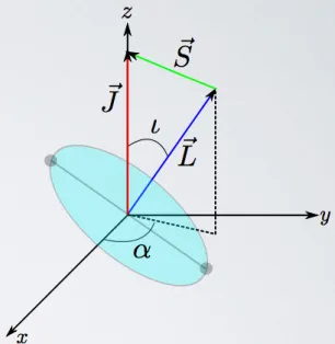
(27) Figure 3.1:. Total angular momentum J as the sum of L and S = S1 + S2 .. Source:. http://hyperphysics.phy-astr.gsu.edu/hbase/quantum/vecmod.html.. The angle ◆ between J and L will evolve in time according to SL + L cos◆ = q , Sp2 + (SL + L)2. (3.23). where SL and Sp are the projections normal and parallel to L. This will lead to simple precession (when J is preserved) or transitional precession (when J changes and eventually goes through zero).. Alfred Castro. 15.


(29) Chapter. 4. Mathematical Procedure Beyond the inspiral, the merger and ringdown of a binary black hole coalescence and computing the gravitational radiation emitted requires numerical simulations to model these stages where both black holes plunge together and ends forming a single Kerr black hole. But such a numerical simulation consists in evolving in time a set of equations that carry information about the spatial structure for a given initial data. However, the Einstein field equations (1.2) are written in a co-variant way, where no distinction between space and time is made and the whole set of coordinates is treated the same way, a formalism to separate the coordinates in a way that allow us to obtain the evolution needs to be done. There are di↵erent approaches to separate Einstein field equations in a way that we can perform a numerical evolution from given initial data, specific formalisms di↵er in the way that the separation is carried out. In this section we will focus in the 3+1 formalism, which is the most used in numerical relativity, but not the only one [21, 22].. 4.1. Initial Value Problem. The aim of this section is to write the Einstein field equations as an initial value problem, i.e. find a solution u(t, x) for all t from a given u(0, x). The 3+1 formalism leads to a set of evolution equations which are not unique. Di↵erent systems of 3+1 evolution equations will have the same physical solution but they will di↵er in their mathematical properties. Our goal is to find a system of equations that is well behaved both mathematically and numerically. In order to achieve that, it has been found that the whole system of evolution 17.

(30) equations has to be well-posed.. 4.1.1. Well-posedness. Once the Einstein field equations are written as an initial value problem, we want it to be well-posed. If appropiate initial data u(0) is defined at t = 0, then, in a well-posed system a unique solution can be found for all the posterior times u(t), and it depends continuously on the given initial data, i.e. ku(t)k  Keat ku(0)k ,. (4.1). where K and a are constants that do not depend on the initial data. For a deeper insight see [23].. 4.2. The 3+1 Decomposition. Global hyperbolicity. We call a Cauchy hypersurface to an hypersurface ⌃ which domain of dependence is the whole space-time M, D(⌃) = M; a space-time which possesses. a Cauchy hypersurface is called globally hyperbolic. Then, if M is globally hyperbolic, it allows a global time function t, such that each surface of constant t is a Cauchy surface; i.e. M can be foliated in surfaces ⌃t , see [24]. To write the Einstein field equations as a Cauchy problem, we start from a 4-dimensional globally hyperbolic space-time M where the metric gab measures coordinate distance between two space-time events,. ds2 = gab dxa dxb ,. (4.2). and the curvature is measured using the notion of parallel transport leading to the Riemann tensor Rabcd . The idea of the 3+1 formalism is to split the 4-dimensional space-time M into a family. of 3-dimensional space-like hypersurfaces of constant t, and see how the evolution variables of this formulation, the induced 3-dimensional metric and the extrinsic curvature, change. in time. The description of how the 3 + 1 decomposition is performed will follow the discussion given by Alcubierre in [25] in parallel with [26]. 18. Alfred Castro.

(31) Figure 4.1: Space-time M split into 3-dimensional hypersurfaces of constant t. Source:[27].. As well as the metric gab measures the distance between two events in the space-time, one uses the 3-dimensional metric. ij. to measure distances within the hypersurface ⌃t. itself, dl2 =. ij dx. i. dxj ,. (4.3). note the use of Latin indices to denote spatial coordinates. Again, analogously to gab , we also use. ij. to raise and lower indices of pure spatial tensors.. We have to define two additional objects to move between di↵erent spatial hypersurfaces and cover the whole space-time: the lapse function ↵(t, xi ) which measures proper time between two hypersurfaces along na , that is a time-like vector normal to the hypersurface, d⌧ = ↵(t, xi )dt, and the shift vector. i. (4.4). , which is a vector tangent to ⌃t that measures the relative velocity. between Eulerian observers (moving along na ) and observers following a coordinate line (where dxi = 0), Figure 4.2. Alfred Castro. 19.

(32) Figure 4.2: Visual definitions of the lapse function and the shift vector. Source:[25].. The unit vector na normal to the spatial hypersurfaces can be expressed in terms of the global time function t as, na =. ↵g ab rb t,. (4.5). where the minus sign indicates that na is pointing upward. It’s normalized in such a way that the lapse function gets the form, na na =. 1 = ↵2 g ab (ra t)(rb t), ↵ = ( g ab (ra t)(rb t)). 1/2. ,. (4.6). an expression for the shift vector can be found, since it’s orthogonal to na , so it lies in ⌃t , i. =. ↵(na · rxi ),. (4.7). the most general way to go from one spatial hypersurface ⌃t to another ⌃t+dt would be, ta = ↵na +. a. .. (4.8). Both the lapse function and the shift vector can be freely specified and they are not unique. Our choice of the lapse will determine the slicing of the space-time just as the shift vector determines the spatial coordinates. They are known as the gauge functions. The line element of the space-time in terms of the functions {↵, ds2 = gab dxa dxb = 20. ↵2 dt +. ij (dx. i. +. i. dt)(dxj +. i. j. ,. ij }. dt),. takes the form, (4.9) Alfred Castro.

(33) and the components of the space-time metric as, ↵2 +. gab =. k. k. j. i ij. !. .. (4.10). Once the space-time is foliated we would like to project the Einstein equations into ⌃t to get the equations to evolve. We have to define a projection operator which is orthogonal to na , and it is nothing more than the induced 3-dimensional metric in each hypersurface by the full space-time metric, ab. = gab + na nb ,. (4.11). then, for example, if we want to define a co-variant derivative into ⌃t (Da ), that will do the same job in the spatial hypersurface that ra does in the space-time, we would have to project every single index of the full space-time co-variant derivative as follows, Da Tcb =. d b f e a e c rd T f ,. (4.12). now Da is a spatial tensor that defines the co-variant derivative into each spatial slice of the space-time, and it’s compatible with the spatial metric Da. bc. = 0, as the co-variant. derivative is with the metric ra gbc = 0.. 4.2.1. Extrinsic Curvature. At this point, we have to distinguish between the intrinsic curvature coming from the internal space-time structure, defined by the Riemann tensor in terms of the 3-dimensional metric. ab .. And the extrinsic curvature, that comes from the way that the spatial hyper-. surfaces ⌃t are embedded in the 4-dimensional space-time. The extrinsic curvature measures the change of the normal vector na when it is paralleltransported from one point in ⌃t to another. So the spatial co-variant derivative of na , Kab =. c d a b rc n d ,. (4.13). will define this variation. Introducing the expression for the projection operator, Kab = =. (gac + na nc )(gbd + nb nd )rc nd , ra n b. (4.14). n a n c rc n b ,. where nd rc nd = 0 because of the normalization. Alfred Castro. 21.

(34) Equivalently, the extrinsic curvature can be written as the Lie derivative of the spatial metric along the normal direction. Finding that it can be seen as the velocity of. ab. seen. by an Eulerian observer, £n a. ab. = n c rc. ab. +. cb ra n. c. +. ac rb n. c. ,. (4.15). = nc rc (gab + na nb ) + (gcb + nc nb )ra nc + (gab + na nc )rb nc , = 2(ra nb + na nc rc nb ), =. 2Kab .. So the extrinsic curvature takes the form, Kab =. 4.2.2. 1 £n a 2. ab .. (4.16). Decomposition of the Riemann tensor. We want to relate 4-dimensional (4) Rabcd to 3-dimensional (Rabcd ,Kab ), note the superscript to denote that we refer to a whole space-time quantity. We consider, (4). Rabcd = gap gbq gcr gds (4) Rpqrs =( =. p a. na np )(. q b. nb nq )(. r c. nc nr )(. s d. nd ns )(4) Rpqrs. p q r s (4) Rpqrs + a b c d. (4.17). p q r s(4) Rpqrs + a b c nd n. +. (4.18). p q r s(4) Rpqrs a b nc n nd n. (4.19). + ..., the other terms would be zero because of the symmetries of Rabcd . We see that there are three di↵erent projections of the Riemann tensor (4.17, 4.18, 4.19) that would lead to the di↵erent equations: Gauss, Codazzi and Ricci equations. Constraints Taking equation (4.17) we can define Gauss’ equation as, p q r s (4) Rpqrs a b c d. 22. = Rabcd + Kac Kbd. Kad Kcb ,. (4.20) Alfred Castro.

(35) that relates the intrinsic curvature of the embedded space to the intrinsic curvature of the embedding space using the extrinsic curvature. If we contract (4.20) with pr q s (4) Rpqrs b d. with. bd. ab. we get,. Kdc Kcb ,. = Rbd + KKbd. where we have introduced the trace of Kab , K =. ac. (4.21). Kab . Now we can contract once more. and we get, pr qs(4). Introducing the definition of. ab. Rpqrs = R + K 2. Kab K ab .. (4.22). (4.11), and working out the term of the LHS,. pr qs(4). Rpqrs = 2np nr Gpr ,. (4.23). where Gpr is the Einstein tensor. So, in terms of the energy density ⇢ = np nr Tpr we get to the Hamiltonian constraint, R + K2. Kab K ab = 16⇡⇢.. (4.24). We do the same for the projections (4.18), so we define the Codazzi’s equation that relates the first projection of the Riemann tensor to co-variant derivatives of the extrinsic curvature, p q r s(4) Rpqrs a b cn. = Db Kac. Da Kbc ,. (4.25). similarly, the contractions of Codazzi equation leads to the momentum constraint, Db Kab. Da K = 8⇡Sa ,. where Sa is the momentum density observed by a normal observer, Sa =. (4.26) b c a n Tbc .. Note that equations (4.24, 4.26) don’t contain time derivatives, this is the reason why they are called constraints, they must be satisfied all times. The constraints are also independent of the gauge functions ↵ and. i. , a fact that indicates that they refer purely. to a given hypersurface. Evolution equations Finally we obtain the evolution equations from the projections (4.19) of the 4-dimensional Riemann tensor, that leads to the Ricci’s equation, nd nc Alfred Castro. q r (4) Rdrcq a b. = £na Kab +. 1 Da Db ↵ + Kbc Kac , ↵. (4.27) 23.

(36) introducing the Einstein field equations, Ricci equation leads to, £na Kab =. 1 Da Db ↵ + Rab ↵ ✓. + KKab where Sab =. c d a b Tcd. and S =. ab. 8⇡ Sab. 2Kac Kbc 1 2. ab (S. ◆. ⇢) ,. (4.28). Sab . This equation is not a constraint, since the Lie. derivative denotes a derivative along the normal (time) direction.. 4.3. The York-ADM equations. The commonly known Arnowitt-Deser-Misner (ADM) equations [28], actually non-trivial rewrote by York, are formed by the set of equations (4.16, 4.24, 4.26, 4.28), rewriting the Lie derivative in the form £na = ↵1 (£t £ ~ ), with £t ⌘ @t and expanding the Lie derivative along the shift vector, • Constraints R + K2. Kij K ij = 16⇡⇢,. Di (K ij. (4.29). ij. K) = 8⇡S i .. (4.30). j. + Dj i ,. (4.31). • Evolution @t. ij. =. 2↵Kij + Di. 2Kik Kjk + KKij ) 1 Di Dj ↵ 8⇡↵(Sij ij (S 2 + k @k Kij + Kik @j k + Kkj @i. @t Kij = ↵(Rij. 4.4. ⇢)) k. .. (4.32). The BSSN equations. The set of equations (4.29-4.32) are evolved using a free evolution approach in a numerical simulation, where the constraints equations are solved initially to get proper initial data, then evolve in time solving the evolution equations for. ij. and Kij . However, in numerical. relativity, the ADM equations are only weakly hyperbolic, a fact that leads to the lack of the necessary stability properties for long-term numerical simulations. 24. Alfred Castro.

(37) This problem was solved by Nakamura, Oohara and Kojima [29]. They presented a reformulation of the ADM evolution equations based on a conformal transformation, and Baumgarte and Shapiro showed that this new formulation has far superior stability properties. Known as the BSSN (Baumgarte, Shapiro, Shibata, Nakamura) formulation [30, 31], it is used by most large codes in numerical relativity. This formulation is characterized by introducing a contracted connection term as a new variable, a conformal decomposition of the metric and extrinsic curvature variables, and adding constraints to the evolution equations. Let’s first consider a conformal re-scaling of the spatial metric, ˜ij = where. 4. ij ,. (4.33). is the conformal factor, chosen in a way that the conformal metric has unit. determinant det ˜ij = 1, condition we ask to be satisfied during the evolution. That implies 4. = det. ij. 1/3. .. (4.34). In practice, one works with the logarithm of the conformal factor. = ln. =. 1 12. ln det. ij .. An evolution equation for this new variable can be found using equation (4.31), @t =. 1 (↵K 6. @i i ) +. i. @i .. (4.35). At the same time, in the BSSN formulation, the extrinsic curvature is separated into its trace K and its trace-free part, 1 3. Aij = Kij. ij K,. (4.36). and a conformal re-scaling of the trace-less extrinsic curvature is also done, Ãij = e. 4. Aij .. (4.37). The BSSN formulation also introduces three new variables known as the conformal connection functions defined as, ˜ i = ˜ ij ˜ ijk =. @j ˜ ij ,. (4.38). where ˜ ijk is the Cristo↵el symbol associated with ˜ij . Alfred Castro. 25.

(38) Now we have to find evolution equations for these new variables. An evolution equation for. is already found (4.35), and for the rest of the variables they can be obtained from. the ADM evolution equations, d ˜ij = 2↵Ãij , dt d 1 = ↵K, dt 6 d Ãij = e 4 ( Di Dj ↵ + ↵Rij + 4⇡↵[ ij (S ⇢) 2Sij ])TF dt + ↵(K Ãij 2Ãik Ãkj ), ✓ ◆ d 1 2 i ij K = Di D ↵ + ↵ Ãij Ã + K + 4⇡↵(⇢ + S), dt 3 where d/dt = @t. (4.39) (4.40). (4.41) (4.42). £ ~ and TF denotes the trace-free part in the expression inside.. The co-variant derivatives of the lapse function with respect to the physical metric. ij. can be calculated considering the relation of the Cristo↵el symbols, ˜k = ij. k ij. 2( ik @j +. k j @i. ij. kl. @l ).. (4.43). The Ricci tensor associated to the physical metric can be separated into two contributions, Rij = R̃ij + Rij ,. (4.44). where R̃ij is computed exactly as Rij but using ˜ij instead; and Rij is given by, Rij = 2D̃i D̃j. 2˜ij D̃k D̃k + 4D̃i D̃j. 4˜ij D̃k D̃k ,. (4.45). where D̃i is the co-variant derivative associated to the conformal metric. To get the full set of equations of the BSSN formulations, we still miss an evolution equation for ˜ i , that can be obtained from equations (4.38) and (4.31), so, 1 2 + ˜ ij @j @k k + j @j ˜ i ˜ j @j i + ˜ i @j j 2(↵@j Ãij + Ãij @j ↵), (4.46) 3 3 that can be written in a more compact way, 1 d ˜i = ˜ ik @j @k i + ˜ ij @j @k k 2(↵@j Ãij + Ãij @j ↵). (4.47) dt 3 But in a numerical evolution, this equation is still unstable. A key step of the BSSN @t ˜ i = ˜ jk @j @k. i. formulation is to use the momentum constraint to fix the instability of this equation. The momentum constraint (4.26) in terms of the new variables takes the form, @j Ãij = 26. ˜ ijk Ãjk. 2 6ãij @j + ˜ ij @j K + 8⇡ j̃ i , 3. (4.48) Alfred Castro.

(39) where j̃ i = e4 j i . So, introducing this equation to (4.47) we obtain, ✓ d ˜i 1 jk i k ij = ˜ @j @k + ˜ ij@j @k 2Ã @j ↵ + 2↵ ˜ ijk Ãjk + 6Ãij @j dt 3. 2 ij ˜ @j K 3. 8⇡ j̃. i. ◆. .. (4.49). The final system of evolution equations is formed by (4.39-4.42) and (4.49). This are known as the BSSN equations that have a big advantage with respect to the YorkADM [32] equations (4.29-4.32), BSSN equations lead to a well-posed initial value problem. The BSSN equations are the currently most widely used form of Einstein’s equations in numerical relativity. Our aim now, is to stably evolve these equations using the numerical code described in the next chapter. However, in order to do that, well-posedness may not be enough. A good choice for the coordinate conditions is also required, i.e., for the lapse ↵ (4.6) and shift. i. (4.7). Useful choices for these gauge conditions must keep an event horizon of a controled size, so it not grows out of the numerical domain; and to find symmetries. Suitable options for these conditions are: (i) a specific choice of the Bona-Masso family for the lapse; (ii) and a Gamma-freezing condition for the shift.. Alfred Castro. 27.


(41) Chapter. 5. Numerical Procedure The need of evolving numerically the Einstein field equations during the last orbits of a binary black hole coalescence, which fall into the strongly dynamic and non-linear regime of General Relativity, has led to the writing of several numerical codes to simulate such an evolution: BAM [33], Einstein ToolKit [34] which is based on the Cactus framework, LEAN [35]... In this thesis we will focus on the BAM code, that is an MPI parallelized code that uses the moving puncture method (see Sec. 5.1) to simulate black hole space-times without excision, and moving boxes mesh refinement, via a free evolution approach.. 5.1. Initial Data. Before starting with the evolution, we need the initial data to be evolved. The initial data consist in the 3-dimensional metric and the extrinsic curvature (. ij , Kij ). induced on. a space-time hypersurface ⌃t , both related by (4.16). This section will be described closely following [33]. One must be especially careful with the description of space-time singularities. As we have already discussed (Chapter 2) the space-time singularities are found where metric components vanish or they diverge. One approach to avoid problems associated with physical singularities is known as the moving puncture method, that is the one used in BAM. Based on modelling each black hole by adopting the Brill-Lindquist wormhole topology. The asymptotically flat end is compactified to a single point r on R3 which is referred to as puncture. The gauge conditions change the wormhole to a trumpet geometry during the 29.

(42) evolution that allows the black hole singularities to be hidden by the punctures because of the discrete structure of the numerical grid. Another used technique is the excision, where a portion of the space-time inside the event horizon is not evolved. This should not a↵ect the solution because of the properties of the event horizon, no physics inside the horizon can influence the outside of it. Proper initial data must satisfy the Einstein constraints and give a realistic representation of the physical system under study. The construction of such an initial data consists of a conformal transformation of the spatial metric and a conformal trace-less split of the extrinsic curvature, ij. =. Kij =. 4 0 ˜ij , 0. 10. (5.1) 1 3. Āij +. ij K,. (5.2). where Āij is trace free. Initially we require a flat metric ˜ij =. ij ;. and the trace of the extrinsic curvature to. be null K = 0, choice corresponding to a maximal slice, that decouples Hamiltonian from momentum constraints and form a set of equations for Āij . The simplest solution for these equations is the trivial one Āij = 0. In addition, in the case of conformal flatness and maximal slice, the momentum constraint takes the simple form of, @j Āij = 0,. (5.3). and admits the Bowen-York solutions. The Hamiltonian constraint, in the conformal flatness, K = 0 and the Bowen-York solution for (5.3), becomes an elliptic equation for the conformal factor, ˜. 0. 1 + K ij Kij 8. 0. 7. = 0,. (5.4). where ˜ is the Laplace operator associated with the flat metric. This equation is often solved by decomposing the conformal factor into a Brill-Lindquist contribution plus a regular contribution u which is determined by an elliptic equation on R3 and is C 1 everywhere except at the punctures where is C 2 , 0. BL. 30. =. BL. =1+. + u, N X mi , 2r i i=1. (5.5) (5.6). Alfred Castro.

(43) where we sum over N possible initial black holes, with mi that parametrizes the mass of each black hole, equal to the total mass only in a Schwarzschild space-time. In the general case, the ADM mass of the ith puncture is given by, Mi = m i. X mj 1 + ui + 2dij i6=j. !. ,. (5.7). where ui is the value of u at the ith puncture, and dij is the coordinate distance between the punctures. This quantity agrees within numerical uncertainty with the apparent horizon mass MAH,i for non-spinning punctures; in the case of spinning punctures it agrees with the black hole mass given by the Christodoulou formula, 2 Mi2 = MAH,i +. Si2 . 2 4MAH.i. (5.8). The ingredients left to complete the initial data are the values of the gauge quantities in the spatial hypersurface ⌃t when t = 0. Choices for the lapse function and the shift vector that have been successfully used are, ↵=1 i. or. ↵=. 0. 2. ,. = 0,. (5.9) (5.10). both to be updated at every time-step following the evolution equations.. 5.2. Evolution. To evolve the described initial data with the evolution equations due to BSSN formalism, first we have to relate the variables in the conformal transverse-trace-less decomposition with the BSSN variables. On the initial slice they are related by, = ln Ãij = ˜i = and. ij. 0, 6. (5.11). Āij ,. (5.12). @j ˜ ij ,. (5.13). and K remain unchanged. Once we have the description of the BSSN variables in. the initial spatial hypersurface, these variables are evolved according to the BSSN evolution Alfred Castro. 31.

(44) equations, d ˜ij dt d dt d Ãij dt d K dt d ˜i dt. =. 2↵Ãij ,. (5.14). =. 1 ↵K, 6. (5.15). 4. (5.16). ( Di Dj ↵ + ↵Rij )T F + ↵(K Ãij 2Ãik Ãkj ), ✓ ◆ 1 2 i ij = Di D ↵ + ↵ Ãij Ã + K , 3 1 = ˜ jk @j @k i + ˜ ij@j @k k 2Ãij @j ↵ ✓ 3 ◆ 2 ij i jk ij ˜ + 2↵ ˜ @j K , jk Ã + 6Ã @j 3 =e. (5.17). (5.18). where matter terms have been set to zero. The Lie derivatives with respect tensor quantities that appear in d/dt = @t. £ ~ are given by,. £~ =. k. 1 @k + @k 6. k. ,. £ ~ ˜ij = ˜ij @k ˜ij + ˜ik @j £ ~ Ãij = Ãij @k Ãij + Ãik @j. (5.19) k. + ˜jk @i k. k. + Ãjk @i. k. 2 ˜ij @k k , 3 2 Ãij @k k . 3. (5.20) (5.21). To improve the stability of the simulation, is a common practice to evolve the BSSN evolution system as a partially constrained system, enforcing the algebraic constraints det(. ij ). = 1 and Tr(Ãij ) = 0 at every full or intermediate step. Moreover, the algebraic constraints and the first order di↵erential constraint ˜ i = @j ˜ ij can be used for the source terms without a↵ecting well-posedness. Translated to the BAM code: • Explicitly use ˜ i =. @j ˜ ij instead of the evolved variable ˜ i whenever it appears. undi↵erentiated.. • Algebraic constraints are imposed when the right-hand sides are computed and at the end of each evolution step.. 5.2.1. Conformal factor. In the moving punctures approach, the wormhole topology of the space-time is captured by th conformal factor, that diverges at each puncture 32. ⇠ 1/r. The singularity in the Alfred Castro.

(45) numerical grid is avoided due to the choice of the gauge. In order to evolve the divergent conformal factor two methods have been found to work: the -method and the -method. In the -method our choice of the conformal factor is directly the original BSSN variable , = ln ,. (5.22). so the evolution system remains the same. In the -method a new finite conformal factor at the puncture is defined as, =. 4. ,. (5.23). and a new evolution equation has to be found to replace (5.15), d 2 = (↵K dt 3. 5.2.2. @j. j. ).. (5.24). Gauge conditions. The gauge conditions (↵,. i. ) in both ADM and BSSN evolution systems are freely speci-. fiable. To describe the gauge conditions we have to keep in mind that the choice of them will allow us to avoid the singularity in the numerical grid. In order to achieve that, we let the lapse function and the shift vector to change in time in such a way that the evolution in proper time should be slowed down in regions where hypersurfaces approach a singularity. In the moving puncture method, the standard choice for evolving the lapse function in the BSSN formalism is given by the co-variant form of “1+log” slicing, (@t. i. @i )↵ =. 2↵K.. (5.25). Suitable choices for the shift vector in order to obtain long term stable numerical simulations is evolve. 5.3. i. according to a Gamma-freezing condition, 3 @t i = B i , 4 i @t B = @t ˜ i ⌘B i .. (5.26) (5.27). Numerical Method. To produce the binary black hole simulation we will use the BAM code, whose features focus on the already mentioned moving punctures method to simulate black hole spacetimes without excision and uses the moving boxes mesh refinement. Alfred Castro. 33.

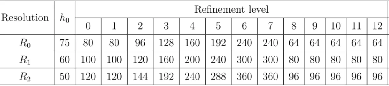
(46) 5.3.1. Evolution Method. To evolve the produced initial data we need two basic ingredients: the evolution system, that we have already described and it leads to the set of the BSSN evolution equations (5.14-5.18); and the discretization algorithm, allowing us to discretize the spatial domain [36]. A suitable numerical algorithm is needed to satisfy the well-posedness of the system. Method of Lines: The BAM code uses the method of lines approach to separate the time and space discretization process. The equations in the 3+1 form are evolved in time using a Runge-Kutta algorithm while the spatial right hand side can be separately discretized. Here a finite di↵erence scheme is used. Artificial Dissipation: In order to avoid high frequency noise from mesh refinement boundaries artificial dissipation terms have been included in the RK4 evolution, even if they are not required for stability. Dissipation terms can be included in the form, @t u ! @t u + Qu,. (5.28). where Q is the Kreiss-Oliger dissipation operator, Q = ( h)2r 1 (D+ )r ⇢(D )r /22r , for a (2r. 2) resolution. Here. (5.29). is a parameter to control the e↵ect of the dissipation. terms, and ⇢ is a weight function currently set to unity.. 5.3.2. Adaptive Mesh Refinement. Black hole space-times involve a wide range of length scales which cannot be efficiently accommodated inside uniform grids and thus require the use of mesh refinement, i.e. a grid resolution that varies in space and time [37]. In the BAM code, a Berger-Oliger type adaptive mesh refinement is implemented [38]. The computational domain consists of a set of nested boxes centered around the individual black holes immersed inside more large boxes containing both black holes. In practice, there are L di↵erent levels of refinement, each labeled by l = 0, . . . , L. 1. One. specific level l consists in a Cartesian grid with constant grid spacing hl . Each grid is completely contained in the next outer level, with grid spacing that di↵ers from the previous 34. Alfred Castro.

(47) one by a factor of 2. So labelling the outermost level with l = 0, with a grid resolution h0 , the resolution at the following levels are hl = h0 /2l , until the innermost level L. 1.. In the case of a binary black hole, when the two punctures are far enough, the hierarchy of the refinement levels consists in non overlapping grids centered in each black hole, boxes in 3D. The size of each box is given by hl ⇥ Nl , where hl is the resolution of the level l, and Nl is the number of discrete points in that level. When the boxes of both black. holes overlap, they are replaced by their bounding box, the smallest rectangular box that contains the two original boxes. The hierarchy of the boxes evolves as the puncture moves. The position of a puncture is tracked using the Crank-Nicholson method by integrating [39], @t xipunc =. i. (xipunc ).. (5.30). The outermost level L = 0 and some of the following finer levels are boxes with a fixed size centered at the origin to avoid unnecessary grid motion.. Figure 5.1: Example of a two dimensional domain. Three di↵erent levels are shown. The two boxes fixed of resolution h0 and h1 are labeled by ”a” and ”b”; and the two boxes ”c” and ”d” of resolution h2 would represent the moving boxes around each black hole. Source: [40].. 5.3.3. Extraction quantities. In each spatial hypersurface, physical information about the binary black hole simulation is extracted. To have a good notion of the quality of the simulation a key step is a Alfred Castro. 35.

(48) good understanding of the results rather than solving the two body problem itself. Some diagnostics quantities and how does BAM compute them is described here. Gravitational Waves: The di↵erence between the Newtonian theory and General Relativity in the two body problem is that in GR the system radiates energy in the form of gravitational waves. The most commonly used approach to extract gravitational waves from black hole binaries simulations is the Newman-Penrose formalism. A description of how the BAM code computes the waveforms as well as the radiated momenta and energy from the knowledge of. ij. and Kij of ⌃t is provided.. The Newman-Penrose scalar is defined as, 4. =. (4). Rabcd na m̄b nc m̄d ,. (5.31). where Rabcd is the Riemann tensor of the 4-dimensional space-time; n and m̄ form part of a null-tetrad l, n, m, m̄ where l and n denote ingoing and outgoing null-vectors. The complex value m̄ is constructed out of two spatial vectors orthogonal to l and n such that, l · n = m · m̄ = 1,. (5.32). with all other inner products between 4-vectors vanishing. The tetrad vector are given by, ✓ i ◆ 1 1 0 i i n =p n =p v , (5.33) ↵ 2↵ 2 ✓ i ◆ 1 1 0 i i l =p l =p +v , (5.34) ↵ 2↵ 2 1 (5.35) m0 = 0 mi = p ui + iwi , 2 where na is the normal vector to the spatial hypersurface; and (ui , v i , wi ) form an orthonormal spatial basis constructed using the Gram-Schmidt method, that in Cartesian coordinates take the form, ui = ( x, y, 0),. (5.36). v i = (x, y, z),. (5.37). wi = g ia ✏abc ub v c .. (5.38). In order to compute the Newman-Penrose scalar in a spatial hypersurface, we need to express it in terms of 3-dimensional quantities in that hypersurface and the spatial 36. Alfred Castro.

(49) vectors described above. We project the 4-dimensional Riemann tensor to get the following relations, associated to Gauss and Codazzi equations (4.20,4.25), p q r s (4) Rpqrs a b c d. = Rabcd + Kac Kbd. p q r s(4) Rpqrs a b cn. = Db Kac. pr q s (4) Rpqrs b d. Kad Kcb ,. (5.39). Da Kbc ,. = Rbd + KKbd. (5.40). Kdc Kcb ,. (5.41). here we have used the projection operator defined as (4.11). So the Newman-Penrose scalar takes the form, 1 (4) Rabcd v a v c 4 = 4 We can project [41] of spin weight. 4. 2. p q r s(4) Rpqrs v c a b cn. +. pr q s (4) Rpqrs b d. (ub. iwb )(ud. iwd ). (5.42). onto spherical harmonics. s Ylm. defined in terms of Wigner d-functions. 2, obtaining the contribution of the individual modes l, m, Z 2⇡ Z ⇡ 2 2 Alm = hYlm , 4 i = 4 Ylm sin ✓d✓d . 0. (5.43). 0. In principle gravitational wave extraction has to be done at infinity, but in practice the right hand side of (5.43) is evaluated on the Cartesian grid and interpolated onto a sphere of finite extraction radius rext using fifth-order polynomials. The integration over the sphere is performed using the fourth-order Simpson method. However, to reduce computational costs, the symmetry properties of the space-time have to be used. This way, for s = A22 = hY22 2 ,. 4i. =. Z. 0. 2 and l = m = 2, we can rewrite equation (5.43) as, ⌘ 2⇡ Z ⇡/2 ⇣ 2 2 sin ✓d✓d . (5.44) 4 Y22 + 4 Y22 0. It is important to remark that most of the energy is radiated in the l = 2 and |m| = 2 modes.. Often one may be interested in the energy and momenta radiated away in the form of gravitational waves, in terms of the Newman-Penrose scalar we can write them as, " # Z Z t 2 dE r2 = lim (5.45) 4 dt̃ d⌦ , r!1 16⇡ ⌦ dt 1 " # Z Z t 2 dPi r2 = lim li (5.46) 4 dt̃ d⌦ , r!1 16⇡ ⌦ dt 1 ( "Z ✓ Z ! #) ◆ Z t Z t̂ t dJz r2 = lim Re @ , (5.47) 4 dt̃ 4 dt̃dt̂ d⌦ r!1 dt 16⇡ ⌦ 1 1 1 Alfred Castro. 37.

(50) where li = ( sin ✓ cos , of (5.43) as,. sin ✓ sin ,. cos ). Equation (5.45) can be also written in terms 2. 2. dE r = lim 4 r!1 16⇡ dt. Z. X. t. 1 l,m. 2. 3. Alm dt̃ 5 .. (5.48). Horizons: A key feature that defines a black hole is its event horizon, a region in the space-time that separate the points from which null geodesics can reach the space-time and points from which they cannot [37]. However, to define the event horizon one needs to know the entire history of the space-time. A more convenient definition is used, and that’s the one of apparent horizon. We can define it as the outermost marginally trapped surface on a spatial slice ⌃t , it is defined locally in time in a space-like slice and depends only on data in that slice. Numerical algorithms to compute apparent horizons have been developed [42], as solution of elliptic PDE. Global quantities: For asymptotically flat space-times, the expression for the energymomentum at spatial infinity was given by Arnowitt, Deser and Misner in their Hamiltonian formalism [43]. The expressions can be given as limits of surface integrals defined at finite radius, the surfaces are taken as spheres Sr of radius r. These surface integrals take the form, Z 1 p ij kl E(r) = ( ik,l ij,k ) dSl , 16⇡ Sr Z 1 p i Pj (r) = (Kji j K) dSi , 8⇡ Sr Z 1 m p l i i Jj (r) = ✏jl x (Km K m ) dSi , 8⇡ Sr in terms of the 3-dimensional induced metric. ij. (5.49) (5.50) (5.51). and the extrinsic curvature Kij . Then. the ADM energy MADM and the linear and angular momentum are given as the limit of (5.49-5.51), MADM = lim E(r),. (5.52). Pj = lim Pj (r),. (5.53). Jj = lim Jj (r),. (5.54). r!1 r!1 r!1. 2 and the rest mass can be defined as MR2 = MADM. 38. P. j=1,3. P j Pj . Alfred Castro.

(51) 5.4. Wave equation as a Toy Model for Hyperbolic Equations. To get a feeling of how the evolution code works, let’s consider a similar case to the Einstein’s field equations but simpler: the wave equation. Going through the wave equation in 1+1 dimensions (one spatial dimension + time), will allow us to explore various useful concepts in numerical simulations such as finite di↵erence, characteristic analysis, the Method of Lines for evolving hyperbolic PDE’s, the Courant-Friedrichs-Lewy stability criterion and convergence testing [44, 45]. Let’s start with the wave equation, @2 @2 + = 0, @t2 @x2. 2 =. (5.55). with 2 being the flat space D’Alembertian operator applied to ; and working in units where c = 1. Performing a complete first order reduction we get to the set of evolution equations, @t ⇡ = @x ( + ⇡),. (5.56). @t = @x (⇡ +. (5.57). @t = ⇡ + where. ), ,. (5.58). is the shift vector but in 1D, and the functions ⇡ and ⇡ = @t. are defined by,. @x ,. = @x .. (5.59) (5.60). The wave equation is completely described by equations (5.56) and (5.57), that can be numerically integrated together with (5.58) to get the physical variable . Characteristic analysis: We can rewrite equations (5.56) and (5.57) as an evolution system for a vector such as, @t u + A@x u = u@x , where u = (⇡, )T , and A= Alfred Castro. 1 1. !. ,. (5.61). (5.62) 39.

(52) whose eigenvalues are 1. =. + 1,. (5.63). 2. =. 1,. (5.64). which are distinct and real, corresponding to a strictly hyperbolic system; and has the characteristic variables given by its eigenvectors 1 w = (⇡ 2. , ⇡ + )T ,. (5.65). corresponding to the right going and left going modes of the scalar field. Initial Data: To provide initial data for ⇡(0, x) and (0, x) is equivalent to say that we provide intial data for (0, x) and @t ( (0, x)) in the second order system. The initial data for (0, x) is freely specifiable, in our case we will consider a Gaussian, (0, x) = Ae then, the initial data for ⇡ and. (x x0 )2 2. ,. (5.66). comes from the time and spatial derivatives of . For. ⇡(0, x), we will require ⇡(0, x) = 0 for time-symmetric initial data. For. (0, x), we just. use the equation (5.60), ⇡(0, x) = 0, (0, x) =. (5.67) 2. (x. x0 ) 2. (0, x).. (5.68). Boundary Conditions: Periodic, reflection and outgoing boundary conditions have been implemented and tested. Here we will focus on the last ones since they represent the physical situation better, the initial pulse propagates outside our numerical domain once it reaches its boundaries. To code these radiative boundary conditions we have to set that there is no incoming waves at the boundary. In order to do that, we set to zero the right going mode at the left boundary and the equivalent at the right one. Numerical Algorithm: To evolve such an hyperbolic system, the Method of Lines is used. It consist in discretizing the spatial dimension, using a finite di↵erence scheme, and integrate in time using a Runge-Kutta method. The set of equations to evolve (5.56-5.58) are all of the type @t f = S(f ), 40. (5.69) Alfred Castro.

(53) where S(f ) is a spatial operator applied to f . To discretize the spatial right hand side a equispaced numerical grid is defined, dividing the continuous domain into J discrete points labeled by i = 1, . . . , J; so the discrete domain is now xi = i x. The spatial derivative is given by its centered finite di↵erence schemes, which at second or fourth order are, fi+1 fi 1 + O( x2 ), 2 x fi+2 + 8fi+1 8fi 1 + fi @x f = 12 x @x f =. (5.70) 2. + O( x4 ),. (5.71). respectively. A fourth order Runge-Kutta method is used to integrate the right hand side in time, k1 = S(tn 1 , f n 1 ), t n 1 t k2 = S(tn 1 + ,f + k1 ), 2 2 t n 1 t k3 = S(tn 1 + ,f + k2 ), 2 2 k4 = S(tn 1 + t, f n 1 + tk3 ), t fn = fn 1 + (k1 + 2k2 + 2k3 + k4 ), 6 where f n. 1. (5.72). denotes the function to integrate at the previous time step tn 1 , and f n is the. integrated function at the new time step tn .. Figure 5.2: Visualization of the CFL condition, shaded regions represent physical domain of influence while discrete points represent numerical domain. A spatial three-points centered finite di↵erence scheme for the evolution is shown. Source: http://www.physics.bu↵alo.edu/phy410505/2011/topic3/app2/index.html.. Alfred Castro. 41.

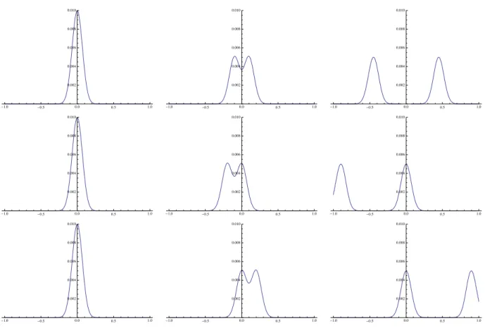
(54) Courant-Friedrichs-Lewy Factor: Is a stability condition named after Richard Courant, Kurt Friedrichs and Hans Lewy [46], required to solve partial di↵erential equations with the Method of Lines. It is a relation between the time step and the spatial step of the form,. c t , (5.73) x where c is the magnitude of the velocity previously set to unity. The physical domain at Cmax. a time tn that influences the next time step tn+1 during the evolution, must be entirely contained in the discretized numerical domain, see Figure 5.2 To evolve the initial Gaussian distribution, the spatial domain was chosen to be [ 1, 1] with a. x = 0.005. The parameters of the initial Gaussian were A = 0.01,. x0 = 0. Di↵erent choices of. -1.0. -1.0. -1.0. -0.5. -0.5. -0.5. and the Courant-Friedrichs-Lewy factor were made.. 0.010. 0.010. 0.010. 0.008. 0.008. 0.008. 0.006. 0.006. 0.006. 0.004. 0.004. 0.004. 0.002. 0.002. 0.002. 0.0. 0.5. 1.0. -1.0. -0.5. 0.0. 0.5. 1.0. -1.0. -0.5. 0.0. 0.010. 0.010. 0.010. 0.008. 0.008. 0.008. 0.006. 0.006. 0.006. 0.004. 0.004. 0.004. 0.002. 0.002. 0.002. 0.0. 0.5. 1.0. -1.0. -0.5. 0.0. 0.5. 1.0. -1.0. -0.5. 0.0. 0.010. 0.010. 0.010. 0.008. 0.008. 0.008. 0.006. 0.006. 0.006. 0.004. 0.004. 0.004. 0.002. 0.002. 0.002. 0.0. 0.5. = 0.1 and. 1.0. -1.0. -0.5. 0.0. 0.5. 1.0. -1.0. -0.5. 0.0. 0.5. 1.0. 0.5. 1.0. 0.5. 1.0. Figure 5.3: Snapshots of the evolution of the initial Gaussian at di↵erent time steps. Di↵erent choices of the coordinate system corresponding to di↵erent. are shown. We use radiative. boundary conditions, the wave propagates out of the domain as it reaches the boundary.. As already discussed in Chapter 4, the choice of the gauge quantity 42. determines our Alfred Castro.

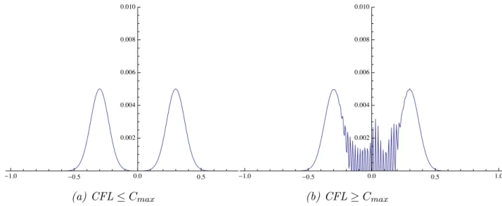
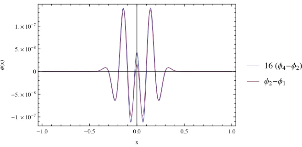
(55) choice of coordinates. In this case, since we are evolving the wave equation in just one spatial dimension, we have set. = [0, 1, 1] to see how di↵erent frames are chosen, see. Figure 5.3. With the value of. = 0, the reference frame is fixed in the middle of the. numerical domain, set to [ 1, 1]; but with the values of. =. 1, 1, that corresponds to. the speed of light, the reference frame is co-moving with the wave that propagates to the left and to the right respectively. Later, in the code where the Einstein field equations are solved, a suitable choice for this quantity would allow us to freeze the horizon of the black hole in place. To converge to a stable solution, the Courant-Friedrichs-Lewy factor can be derived p analytically as Cmax = 8 [46]. Evolving the wave equation with C larger than Cmax will lead to high frequency numerical instabilities that grow faster with higher resolution, they appear in the code as shown in Figure 5.4.. -1.0. -0.5. 0.010. 0.010. 0.008. 0.008. 0.006. 0.006. 0.004. 0.004. 0.002. 0.002. 0.0. (a) CFL  Cmax. 0.5. -1.0. 1.0. -0.5. (b) CFL. 0.0. 1.0. 0.5. Cmax. Figure 5.4: Snapshots of the evolution of the initial Gaussian at a certain value of t. If the Courant-Friedrichs-Lewy condition (5.73) is not fulfilled, instabilities in the solution appear.. Moreover, it will be useful to perform a convergence test over the found solution to check the validity and accuracy of the solution. In this case, where both the time integrator and the finite di↵erence stencil for the spatial derivative, is fourth order, we expect a fourth order convergence. To check that, we evaluate di↵erences between the solution computed at di↵erent resolutions (see Sec. 6.1.1 for a detailed explanation). One have to take care of evaluate the solution in the di↵erent resolutions at the same point in the domain. In Figure 5.5, we see that the di↵erences agree with fourth order convergence. Alfred Castro. 43.

(56) 1. ¥ 10-7. fHxL. 5. ¥ 10-8. 16 Hf4 -f2 L. 0. f2 -f1 -5. ¥ 10-8 -1. ¥ 10-7 -1.0. -0.5. 0.0. 0.5. 1.0. x. Figure 5.5: Convergence results for the wave equation after 10 temporal iterations. Solution shows fourth order convergence.. To evolve the Einstein field equations in the BSSN form, we have to take into account the considerations mentioned above. The evolution will be performed with the BAM code in the next section.. 44. Alfred Castro.

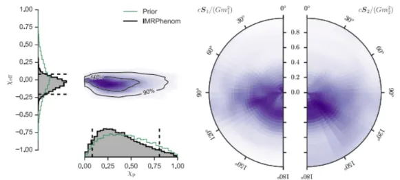
(57) Chapter. 6. Numerical Simulations of a Precessing q = 1.2 Black Hole Binary The role of Numerical Relativity begins after the binary has gone through a slow inspiral phase modeled by analytical approximations such as the e↵ective one-body approach. When the fully general relativistic numerical evolution starts, the initial inspiral stage took care of reducing the eccentricity of the orbits via the emission of gravitational waves. The integration of the post-Newtonian equations of motion in the e↵ective one-body form in done over hundreds of orbits from an initial large separation until the binary reaches such separation that only a few orbits remain to the merger. The reason to start the integration of the PN equations from this large separation is to let the radiation reaction circularize the orbits [47]. In this case, we study a q = M2 /M1 = 1.2 [10] binary system, where M1 and M2 are the black hole individual masses (see Figure 6.1). The integration of the Post-Newtonian equations is done from an initial separation of r = 40M , where M = M1 + M2 ; note that both distance and time are scaled with the total mass M . We use Mathematica [48] to evolve during a time of approximately 224 158M . In this time, the binary completes around 455 orbits and reaches a separation of r = 10.62M . This will be the starting point for the simulation code to accurately simulate the last 5 orbits; the merger, which is estimated to occur after around 1200M ; the ringdown of the system and the gravitational waves emitted. Opposed to the mass distribution, the spin distribution shows that the spin components are poorly constrained, see Figure 6.2. Specifically, the component that is responsible of 45.

(58) Figure 6.1: Probability distributions for the masses M1 and M2 for the individual black holes. Source: [10]. the precession. p,. is compatible with. p. = 0 but also with. p. ⇡ 1. In this thesis, we choose. a precessing configuration (Table 6.1) to show that it is also consistent with GW150914, p. is taken to be. 6.1. p. ⇡ 0.2. Runs Configuration. The simulations were carried out in the BSC-CNS Marenostrum supercomputer [49] using the BAM code. The BSC-CNS Marenostrum is a supercomputer with a peak performance of 1.1 Petaflops; it consists in 2880 nodes with 16 cores per node of 2Gb/core of RAM memory, and 256 nodes with also 16 cores per node of higher memory cores. As stated, the starting point will be where the integration of the PN equations finishes. There, parameters of the punctures, which define the initial black holes, are summed up in Table 6.1. 46. Alfred Castro.