Electrodeposition of nickel nanoparticles and their characterization

Texto completo

(1)

(2) c Gerardo Tadeo Martínez Alanis, 2006.

(3) Electrodeposition of Nickel Nanoparticles and their Characterization por. Ing. Gerardo Tadeo Martínez Alanis. Tesis Presentada al Programa de Graduados de la Escuela de Tecnologías de Información y Electrónica como requisito parcial para obtener el grado académico de. Maestro en Ciencias especialidad en. Sistemas Electrónicos. Instituto Tecnológico y de Estudios Superiores de Monterrey Campus Monterrey Diciembre de 2006.

(4) Instituto Tecnológico y de Estudios Superiores de Monterrey Campus Monterrey Escuela de Tecnologías de Información y Electrónica Programa de Graduados en Tecnologías de Información y Electrónica. Los miembros del comité de tesis recomendamos que la presente tesis del Ing.Gerardo Tadeo Martínez Alanis sea aceptada como requisito parcial para obtener el grado académico de Maestro en Ciencias, especialidad en: Sistemas Electrónicos. Comité de tesis:. Dr. Genaro Zavala Enriquez. Dr. Marcelo Videa Vargas. Asesor de la tesis. Co-Asesor de la tesis. Dr. Alejandro Javier García Cuéllar. Dr. Omar Yague Murillo. Sinodal. Sinodal. Dr. David Garza Salazar Director del Programa de Graduados en Tecnologías de Información y Electrónica. Diciembre de 2006.

(5) A mis padres, Gerardo y Cristina, A mis abuelos, Evelio y Ana María, Miguel y Luz, A mis hermanos, Pablo, Montserrat y Fatima.. ...The Blind See...-The Way to Love.

(6) Reconocimientos. Al CONACyT y al Tecnológico de Monterrey, por su apoyo …nanciero a traves de las Becas de Excelencia y las Cátedras de Investigación CAT-007 y CAT-051. A mis asesores, Dr. Genaro Zavala y Dr. Marcelo Videa, por sus enseñanzas, discusiones, esfuerzo y paciencia. A mis sinodales, Dr. Alejandro García y Dr. Omar Yague, por complementar mi trabajo con sus observaciones a esta tesis. Al Dr. Julio Gutiérrez por su apoyo durante mi investigación. Al Dr. Alex de Lozanne y Changbae Hyun por su apoyo en las mediciones magnéticas mediante SQUID. A la Ing. Lorena Cruz, por invitarme a conocer la ciencia de la microscopía, por sus consejos y aportaciones. Al Lic. Jorge Lozano y a Residencias del Campus Monterrey, por brindarme un hogar durante mi estancia en este Instituto, por su apoyo y aprendizajes. A la Lic. Victoria Medina, por creer en mi desde el principio. A mis compañeros de Laboratorio, en especial al Lic. Joaquín Rodríguez. A mis colegas IFIs, por su amistad, apoyo y tiempo compartido. En especial a Poncho, Rodolfo, Yilen y Omar, por su ayuda en la obtención de información relevante para esta investigación. A la Comunidad, por su sincera amistad. A Martha, por todo lo que crecimos juntos durante este tiempo. A mi familia, por su amor incondicional. A la Vida por permitirme concluir esta tesis, y con ella, una etapa más de mi crecimiento personal y profesional.. Gerardo Tadeo Martínez Alanis Instituto Tecnológico y de Estudios Superiores de Monterrey Diciembre 2006.

(7) Electrodeposition of Nickel Nanoparticles and their Characterization. Gerardo Tadeo Martínez Alanis, M.C. Instituto Tecnológico y de Estudios Superiores de Monterrey, 2006. Advisor: Dr. Genaro Zavala Enriquez Co-advisor: Dr. Marcelo Videa Vargas. Electrodeposition of nickel nanoparticles on indium tin oxide (ITO) substrate is achieved by an alternative electrochemical method in which pulsed current is applied. Determination of the nucleation mechanism of the particles by comparison to theoretical model using one potential step is presented. The critical nucleation potential was found to be 800 mV with respect to Ag/AgCl reference electrode and the the nucleation mechanism resulted to be instantaneous nucleation. The pulsed current technique results are discussed considering variables such as pulsed current duration, pulsed current intensity and …xed transferred charge. Topographical characterization of the particles was carried out by Atomic Force Microscopy (AFM) and Scanning Electron Microscopy (SEM). Particles between 50 300 nm were obtained, showing di¤erent crystallization types. Magnetic characterization by Magnetic Force Microscopy (MFM) and Superconducting Quantum Interference Device (SQUID) magnetometry showed that the particles of 50 100 300 nm were ferromagnetic with a coercive …eld of 200 Oe and a saturation magnetization of 3:6 10 4 , 2 10 4 and 4 10 5 emu at 300 K, respectively. They can be magnetized in single magnetic domains..

(8) Contents. List of Figures. iii. List of Tables. ix. Chapter 1 Introduction. 1. 1.1 1.2 1.3 1.4. Nanoparticle De…nition . . . . . . . . . . . . . . . . . . . . Preparation Methods of Nanoparticles . . . . . . . . . . . Electrodeposition of Nanoparticles . . . . . . . . . . . . . . Nucleation of Nanoparticles . . . . . . . . . . . . . . . . . 1.4.1 Homogeneous Nucleation . . . . . . . . . . . . . . . 1.4.2 Heterogeneous nucleation . . . . . . . . . . . . . . . 1.4.3 Models of Nucleation Process . . . . . . . . . . . . 1.5 Nucleation by the In‡uence of an Overpotential . . . . . . 1.5.1 Di¤usion Controlled Growth under the In‡uence of tential . . . . . . . . . . . . . . . . . . . . . . . . . 1.5.2 The Double Pulsed Potential Method . . . . . . . . 1.6 Particle Characterization Techniques . . . . . . . . . . . . 1.6.1 Topographic Characterization . . . . . . . . . . . . 1.6.2 Magnetic Characterization . . . . . . . . . . . . . .. . . . . . . . . . . . . . . . . . . . . . . . . . . . . . . . . . . . . . . . . . . . . . . . . . . . . . . . . an Overpo. . . . . . . . . . . . . . . . . . . . . . . . . . . . . . . . . . .. Chapter 2 Experimental Setup. 20 25 27 29 36 48. 2.1 Electrochemical cell . . . . . . . . . . . . . . . . . . . . . . . . . . . . . 2.2 Electrodeposition Experiments . . . . . . . . . . . . . . . . . . . . . . . 2.3 Characterization . . . . . . . . . . . . . . . . . . . . . . . . . . . . . . Chapter 3 Results and Discussion 3.1 3.2 3.3 3.4. 6 7 9 9 10 15 17 17. 48 51 55 61. Substrate Characterization . . . . . . . . . . Determination of the Nucleation Mechanism Pulsed Current Experiments with Respect to Pulsed Current Experiments with Respect to i. . . . . . . . . . . . . . . . . . . Time . . . . . Pulse Intensity. . . . .. . . . .. . . . .. . . . .. . . . .. . . . .. 61 62 71 76.

(9) 3.5 Pulsed Current Experiments at Constant Transferred Charge . . . . . . 3.6 Topographic Characterization . . . . . . . . . . . . . . . . . . . . . . . 3.7 Magnetic Characterization . . . . . . . . . . . . . . . . . . . . . . . . .. 83 91 99. Chapter 4 Conclusions. 107. Appendix. 111. Bibliography. 118. Vita. 123. ii.

(10) List of Figures. 1.1 Brief history of key schemes, devices and theories of present magnetic recording [5] . . . . . . . . . . . . . . . . . . . . . . . . . . . . . . . . . 1.2 Development of magnetic recording to the video and digital information in the later half of the 20th century [5] . . . . . . . . . . . . . . . . . . 1.3 Rate of increase in areal density is slowing signi…cantly. For conventional recording technology, fundamental issues force trade-o¤ among: “Writability”, “Signal-to-Noise”, “Thermal Stability”[6] . . . . . . . . 1.4 Examples of zero-dimensional nanostructures or nanomaterials with their typical ranges of dimension [12]. . . . . . . . . . . . . . . . . . . . . . . 1.5 Typical three electrode electrochemical cell used for electrodeposition. The electrodes are Working Electrode (WE), Reference Electrode (RE) and Counter Electrode (CE). . . . . . . . . . . . . . . . . . . . . . . . . 1.6 Schematic ilustration of the change of volume free energy, v , surface free energy, G; as functions of r [12]. . . . . s and total free energy 1.7 Schematic ilustrating the processes of nucleation and subsequent growth [13]. . . . . . . . . . . . . . . . . . . . . . . . . . . . . . . . . . . . . . 1.8 Schematic illustrating heterogeneous nucleation process with all related surface energy in equilibrium [12] . . . . . . . . . . . . . . . . . . . . . 1.9 Schematic ilustrating three basic modes of inital nucleation in the …lm growth. Island growth occurs when the growth species are more strongly bonded to each other than to the substrate. . . . . . . . . . . . . . . . 2 1.10 Theoretical non-dimensional plots of I 2 =Im vs. t=tm , for (a) instantaneous; and (b) progressive nucleation. . . . . . . . . . . . . . . . . . . . 1.11 Schematic views of the hypothetical di¤usion cylinders around; (a) an established nucleus; and (b) a newly appeared nucleus at successive time intervals after nucleus (b)’s appearance (smallest cylinders to largest cylinders). (A) Sharifker-Mostany Model. (B) Sluyters-Rehbach et al Model. at the top of the cylinders represent bulk solution concentration, the (B) model is formulated to ensure equal di¤usion layer thickness for all nuclei. . . . . . . . . . . . . . . . . . . . . . . . . . . . . . . . . . .. iii. 3 4. 5 7. 10 12 13 16. 18 23. 24.

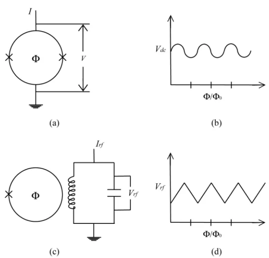
(11) 1.12 Schematic representation of the potentiostatic double-pulse method. After an equilibrium period, a nucleation pulse of potential E1 is applied for a time t1 . To form nucleation sites, E1 must be more negative than a critical nucleation potential ECRIT . The …rst pulse is inmediately followed by a growth pulse of potential E2 for time t2 . As E2 is more positive than ECRIT , no further nucleation on the subtrate is possible. . . . . . . 1.13 SEM images of silver clusters on ITO substrates, deposited with the double pulsed potential method [26]. . . . . . . . . . . . . . . . . . . . 1.14 Schematic of AFM system. The tip approaches the surface while its de‡ection is monitored by a laser beam. The changes in surface topography are manifested in the cantilever de‡ection due to the tip-sample interaction. By means of a feedback loop, the de‡ection is mantained constant by moving the sample using a piezoelectric. The voltages applied to the piezoelectric are then translated to surface topography in nanometers. . 1.15 Schematic of the SEM system. The electron beam is focused by magnetic lenses and it interacts with the sample. Depending on the electron beam-sample interaction, there can be di¤erent signals to be detected, like secondary electrons or backscattered electrons, that give information about the surface morphology. . . . . . . . . . . . . . . . . . . . . . . . 1.16 Ordering of the magnetic dipoles in magnetic materials. . . . . . . . . . 1.17 Magnetization curves for diamagnetic, paramagnetic and antiferromagnetic materials. . . . . . . . . . . . . . . . . . . . . . . . . . . . . . . . 1.18 Magnetization curves for ferri- and ferromagnets. . . . . . . . . . . . . 1.19 Hysteresis loop for a ferro- or ferrimagnet. . . . . . . . . . . . . . . . . 1.20 Typical magnetization behavior of a superparamagnetic material. It can be observed that the magnetic hysteresis loop in this condition does not appear. . . . . . . . . . . . . . . . . . . . . . . . . . . . . . . . . . . . . 1.21 The e¤ect of the force derivative: …rst line from left to right corresponds to the absence of the force derivative; next line corresponds to the presence of the attractive force derivative (positive derivative) [50]. . . . 1.22 The magnetic tip-sample interaction is detected by a phase shift originated in the detected laser signal and the piezoelectric drive phase signal. The phase shift is related to the force gradient [51]. . . . . . . . . . . . 1.23 The Josephson junction in (a) consists of a superconductor such as niobium separated by a thin insulation layer. The volatge (V ) vs. the current (I) curve in (b) shows that a superconducting current ‡ows through the junction with zero volts across the junction [55]. . . . . . .. iv. 26 27. 31. 35 38 39 40 41. 42. 44. 45. 46.

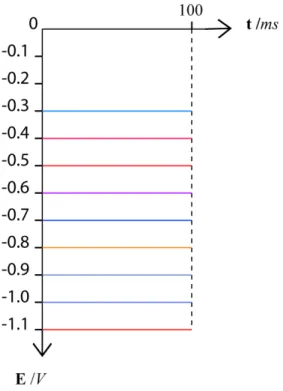
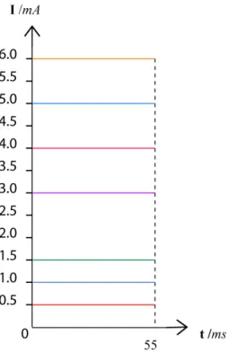
(12) 1.24 (a) Schematic of a dc-SQUID. Two Josephson junctions are shown by in the superconductor ring, (b) Variation of voltage of the dc-SQUID with the applied ‡ux ( ) for a constant bias current, (c) Schematic of a rf-SQUID and (d) variation of peak amplitude of Vrf with with the applied ‡ux ( ) for a …xed rf bias current. . . . . . . . . . . . . . . . . 2.1 Electrochemical cell elements. . . . . . . . . . . . . . . . . . . . . . . . 2.2 Experimental setup. The electrochemical cell was built up in a EG&G Princeton Applied Research potentiostat/galvanostat . . . . . . . . . . 2.3 Schematic of one pulsed potential experiments to determine the nucleation mechanism. . . . . . . . . . . . . . . . . . . . . . . . . . . . . . . 2.4 Schematic of equal intensity pulsed current experiments varying the duration of the pulsed current. . . . . . . . . . . . . . . . . . . . . . . . . . 2.5 Schematic of di¤erent intensity pulsed current for equal period of time. 2.6 Schematic of the pulsed current experiments when transferred charge is kept constant. . . . . . . . . . . . . . . . . . . . . . . . . . . . . . . . . 2.7 Characterization equipment used to obtain the topography and magnetic properties of the nanoparticles. . . . . . . . . . . . . . . . . . . . . . . 2.8 Schematic illustration of random functions with various skewness and kurtosis values [61]. . . . . . . . . . . . . . . . . . . . . . . . . . . . . . 3.1 SEM micrograph of ITO thin …lm on glass substrate before doing the electrodeposition. The image shows that the surface has scratches and small contaminations. . . . . . . . . . . . . . . . . . . . . . . . . . . . . 3.2 SEM micrograph of ITO thin …lm on glass substrate before electrodeposition. At higher magni…cation, the surface is smooth with granular structures and bumps. . . . . . . . . . . . . . . . . . . . . . . . . . . . 3.3 1 m 1 m AFM image of the ITO thin …lm. The image shows that surface is relatively ‡at with small features. . . . . . . . . . . . . . . . 3.4 Current transients after one potential pulse is applied. . . . . . . . . . . 3.5 Transferred charge for each pulsed potential.The lines were drawn as visual aids to see that the behavior of this variable changes at 800 mV. 3.6 Comparison between electrochemical data and the instantaneous nucleation model proposed by Sharifker and Mostany [20] . . . . . . . . . . 3.7 SEM micrograph of Ni particles on an ITO substrate. It can be observed that some particles follow the direction of the scratches on the surface. 3.8 SEM micrograph of Ni particles on an ITO substrate. In this case, the presence of small contamination favors the growth mechanism. . . . . .. v. 47 50 52 53 54 55 56 57 59. 62. 63 64 66 67 67 69 70.

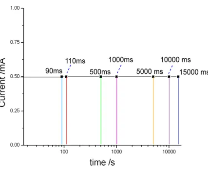
(13) 3.9 Potential behavior after a 0.5 mA pulse is applied to the system. The plot shows several experiments superimposed in which the pulse length is varied from 90 ms to 15000 ms. . . . . . . . . . . . . . . . . . . . . . 3.10 Particle size distribution obtained by SEM image analysis and the schematic of its corresponding polarization plot. It can be observed that the particle size distribution behaves di¤erently depending on the duration of the pulse. For short periods of time, the Lorentzian curve does not …t accurately, meanwhile for long periods this probability density function …ts the particle size distribution more accurately. . . . . . . . . . . . . 3.11 Statistical data of the analyzed SEM images. The particle mean size increases with time, while the particle size dispersion mantains a relation of 20 30% the particle mean size. . . . . . . . . . . . . . . . . . . . . 3.12 Particle density variation during time . . . . . . . . . . . . . . . . . . . 3.13 Schematic of the proposed deposition mechanism for pulsed current. The plots represent the behavior of the induced potential to the system. The schematics below each plot show the nucleation and growth of the particles, in which the gray intensity color of each particle reprents the birth of the nucleus. The order of nucleation is for white, dark gray and light gray respectively. The dashed lines represent the difussion layers. 3.14 Polarization curves when di¤erent intensity pulsed current is applied to the system. The minimum potential value reached on every experiment depends on the intensity of the pulse. . . . . . . . . . . . . . . . . . . . 3.15 Minimum potential values versus pulsed current intensity from Figure 3.14. The behavior of the system shows a linear dependence. . . . . . . 3.16 Inverse of the time required to reach the minimum potential versus current pulsed intensity. The relation of these variables show a linear behavior. 3.17 Particle size distribution plots with their corresponding schematic of pulsed current plot. . . . . . . . . . . . . . . . . . . . . . . . . . . . . . 3.18 Particle size mean with standard deviation for experiments varying the current pulse intensity . . . . . . . . . . . . . . . . . . . . . . . . . . . 3.19 Particle density plot versus pulsed current intensity. The particle density increases as the pulsed current intensity increases . . . . . . . . . . . . 3.20 Relation between the particle mean size and the di¤erence of minimum potential reached by applying the pulsed current with respect to the critical potential Ecrit . . . . . . . . . . . . . . . . . . . . . . . . . . . . 3.21 Polarization curves when di¤erent intensity pulsed current is applied, but keeping the transferred charge constant . . . . . . . . . . . . . . . 3.22 Particle size distribution plots for experiments when the transferred charge was kept constant . . . . . . . . . . . . . . . . . . . . . . . . . .. vi. 71. 73. 74 74. 77. 78 79 79 81 82 82. 84 85 86.

(14) 3.23 Particle size mean with particle size standard deviation for experiments with transferred charge conserved. The particle size decreases for very intense pulsed current . . . . . . . . . . . . . . . . . . . . . . . . . . . 87 3.24 Particle density vs pulsed current intensity plot. The particle density increases with an increasing pulsed current intensity. . . . . . . . . . . 88 3.25 Minimum potential reached vs pulsed current intensity. The relation of these two variables show a linear behavior. . . . . . . . . . . . . . . . . 89 3.26 Inverse of time required to reach the minimum potential versus pulsed current intensity. The behavior was found to be linear. . . . . . . . . . 90 3.27 Particle mean size vs di¤erence of minimum potential reached by applying pulsed current with respect to critical nucleation potential Ecrit . . 91 3.28 Total volume of Ni deposited with respect to pulsed current intensity . 92 3.29 The morfology of the particles was found to have di¤erent crystallization types. . . . . . . . . . . . . . . . . . . . . . . . . . . . . . . . . . . . . 93 3.30 Di¤erent crystallization types of particles were found in the same experiment. The di¤erent crystallization happen under the same electrochemical conditions. . . . . . . . . . . . . . . . . . . . . . . . . . . . . . . . 94 3.31 The morphology of the particles is not determined by local concentration of nickel ions during growth, since two particles may have di¤erent crystallization types, when they grew at short distances, where the depletion layer condiction appears fast. . . . . . . . . . . . . . . . . . . . . . . . 95 3.32 The particle deposition was found to be preferable for irregularities on the surface, such as scratches, when the pulsed current intensity was low. The image was taken from the experiment when a 1.5 mA pulsed current is applied for 55 ms. . . . . . . . . . . . . . . . . . . . . . . . . . . . . 96 3.33 The particle deposition for very intense pulsed current was found to be preferable on the regular surface of the sample, avoiding the irregularties, such as scratches.This image was taken when a 30 mA pulsed current is applied for 1.33 ms . . . . . . . . . . . . . . . . . . . . . . . . . . . . . 97 3.34 Low density and high density particle deposition comparison. The particles maintain a hemispherical morpologhy in spite of the particle density in the substrate . . . . . . . . . . . . . . . . . . . . . . . . . . . . . . . . 100 3.35 MFM images of 300 400 nm sized particles in relaxed state and magnetized state. It can be observed that they are monodomain particles after magnetization . . . . . . . . . . . . . . . . . . . . . . . . . . . . . 101 3.36 MFM images of particles 50 90 nm size. The image contrast is improved after magnetizing the sample. . . . . . . . . . . . . . . . . . . 103 3.37 AFM topography and its corresponding MFM image. It can be observed in zone marked by the white cicle that a few particles couple their magnetization to provide magnetic domains bigger than the particle size . . 104 vii.

(15) 3.38 SQUID measurements of particles 50 nm. They show a ferromagnetic behavior, however, the hysteresis loop starts to show the shape for a superparamagnetic material. . . . . . . . . . . . . . . . . . . . . . . . . 105 3.39 SQUID measurements for particles 100 nm. They show a ferromagnetic behavior. . . . . . . . . . . . . . . . . . . . . . . . . . . . . . . . 106 3.40 SQUID measurements for particles 300 nm. They show a ferromagnetic behavior. . . . . . . . . . . . . . . . . . . . . . . . . . . . . . . . 106 1. 2. 3 4 5. Image histogram. It can be observed that there are more pixels near the black (0) value than in the white (255) value. These pixels are interpreted to be from the substrate, so, a threshold value dividing these regions of pixels allowed to convert the image into binary mode, where the particles remained white and the substrate was converted to black. Example image to be analyzed by the MATLAB program. These image is in binary mode and has a speci…c pattern of particles. It also has some defects (black pixels) on the biggers particles, since during the binary mode conversion, some particles may have these defects due to the threshold value. . . . . . . . . . . . . . . . . . . . . . . . . . . . . Image after dilation process. The particles are 1 pixel bigger, but the 1 pixel black defects dissapear. . . . . . . . . . . . . . . . . . . . . . . . Image after erosion procedure. The particles loose 1 pixel that was added by the dilation process. . . . . . . . . . . . . . . . . . . . . . . . . . . Particle size distribution in pixels of the speci…c pattern image used as example for the image processing programm. . . . . . . . . . . . . . .. viii. 112. 113 114 115 117.

(16) List of Tables. 2.1 Scanning parameters for the obtained MFM images . . . . . . . . . . . 3.1 3.2 3.3 3.4 3.5 3.6. 60. Roughness parameters for ITO thin …lm determined by AFM inspection 61 Results of pulsed potential experiments. . . . . . . . . . . . . . . . . . 65 Particle Size Parameters determined from AFM inspection . . . . . . . 68 Particle aspect ratio found by AFM characterization . . . . . . . . . . . 98 Magnetic properties measured by SQUID . . . . . . . . . . . . . . . . . 102 Saturation Magnetization of the particles . . . . . . . . . . . . . . . . . 104. ix.

(17) Chapter 1. Introduction. I belive that many people in the audience of the Annual Meeting of the American Physical Society back in 1959 where considering Richard Feynman as a great visionary but just making an extraordinay Gedanken exercise (as Einstein used to do) until he said: "...is possible according to the laws of physics" [1]. Then I guess many of them just enjoyed the exercise, but others certainly believed on those words and started to work on the idea of miniaturizing things and searching for the room that is available in the small scales, thinking on all possible applications of atomic technology. I am sure that the ones that heard that talk and survived until today would think that Feynman was just but a gypsy man with a crystal ball predicting the future: a “crystal ball”called faith on the man desire to understand and manipulate its enviroment and certainity on the natural laws of physics. He talked about many things that could be possible to do, but the newcoming researchers dealt with all the technical di¢ culties to achieve this vision, giving the opportunity to a hole new and amazing technology to develop: Nanotechnology. The term Nanotechnology was …rst used by Taniguchi [2] in 1974 to refer to “production technology to get the extra high accuracy and ultra …ne dimensions, i.e. the preciseness and …neness on the order of 1 nm (nanometer), 10 9 meter in length”. From that cite, there have been several modi…cations to the term, becoming more explicit and clear, like the NASA de…nition [3]: “Nanotechnology is the creation of functional materials, devices and systems through control of matter on the nanometer length scale (1-100 nanometers), and exploitation of novel phenomena and properties (physical, chemical, biological, mechanical, electrical...) at that length scale”. This de…nition considers a wide range of possibilities to consider. One of these options is the study of magnetic materials at this scale, emerging the concept of nanomagnetism. According to a review written by S.D. Bader [4], the aim to study nanomagnetism is to (i) create, (ii) explore, and (iii) understand new nanomagnetic materials and phenomena. He proposes some interesting areas of research, as it follows: Ultrastrong permanent magnets 1.

(18) Ultra-High-Density Media Spin Transistor with Gain Nearly 100% Spin-Polarized Materials Room-Temperature Magnetic Semiconductors Instant Boot-Up Computer Spin-based Qubits Hierarchically Assembled Media Nanobiomagnetic Sensors From these areas of research, it is possible to observe the variety of options to study, but one of them has had an increasingly attention due to its relevance in the development of other technologies: Ultra-High-Density Recording Media. This topic is of interest to many industries because all of them have the need to storage their information in a durable and reliable way. The information era we are living in requires better and higher capacity storage media. Today’s media stores almost 100 Gbits/in2 but in order to advance to Tbits/in2 and beyond, new approaches are required, and nanomagnetism might provide what is needed [4]. The aim to study these properties on nanomaterials and …nding a reliable and e¢ cient way to produce them is motivating scientist to their top e¤orts.. Brief History of the Development of Magnetic Recording The …rst magnetic recorder, the “Telegraphone”, was invented by V. Poulsen in 1898 [5] using a steel wire and getting the idea for it from the observation that iron …lings tied together by a geomagnetic …eld. One hundred years of the 20th century can be said to be the history of continuous development that has migrated from wires to tapes to disks. Figure 1.1 shows the times of development of the key devices and theories that are used in current magnetic recording systems, in comparison with the products at those times. In the …rst half of the 20th century, the great evolution from steel wire (tape) recorders to magnetic tape recorders was made by the inventions of the Magnetophone at AEG in 1935. Ring heads, magnetic tape with particulate magnetic materials, and AC biasing method, shown in the left column, are still the basic technologies of present magnetic recording. Moreover, progress in the theory of signal reproduction of magnetic head, namely, the concepts such as spacing loss. 2.

(19) Figure 1.1: Brief history of key schemes, devices and theories of present magnetic recording [5]. 3.

(20) Figure 1.2: Development of magnetic recording to the video and digital information in the later half of the 20th century [5]. and reciprocity principle constributed to the realization of high performance broadcast sound recorders in the latter half of the 1940s. Figure 1.2 shows the development of magnetic recording to video and digital information in the latter half of the 20th century. As indicated on the top of the right column, the …rst broadcast video recorder by AMPEX and digital computer hard disk drive by IBM were produced in 1956 and 1957, respectively. These two products contributed to building the present information technology (IT) world. That is, the inital huge broadcast video recorders using 2-in-wide tape and four heads have transformed to small 8-mm video recorders of helical scan system with two heads. Computer hard disks have also increased their recording density from 2 kb/in2 for RAMAC to the present 10 Gbit/in2 , and have realized a large capacity of 15 GB for a 3.5-in disk. A prototype perpendicular hard disk drive has appeared in the last year of the 20th century. In the left column of Figure 1.2, key devices and theories are depicted as the 4.

(21) Figure 1.3: Rate of increase in areal density is slowing signi…cantly. For conventional recording technology, fundamental issues force trade-o¤ among: “Writability”, “Signalto-Noise”, “Thermal Stability”[6]. motivations of above products. It teaches us that the metal particulate tape which was produced for the 8-mm video recorder, and perpendicular magnetic recording which resulted in the perpendicular hard disk has appeared respectively about 20 years before each realization of the recording equipment. The latter invention was based on the development of vector recording theory by the large-scale model experiment and the self-consistent magnetization model. The MR1 -head-based hard disk drive after 1990 is also the realization of the invention in 1971. As a result, more than 20 years are needed to advance from an invention to reach worldwide application. The development of magnetic recording technology has advanced very fast in the past decades. Recent products exceed 100 Gbit/in2 and with a rate of increase approaching 40% per annum. If this rate were to be sustained over 10 years, we would reach approximately 10 Terabits/in2 . It is far exceeding even the most optimistic projections of the densities that can be supported by conventional technology [6]. Recent advances, however, are very encouraging with respect to our ability to approach 1 Terabit/in2 and the …gure 1.3 shows a simple projection towards this asymptotic value. Recent successful introduction of several important new technologies into products as well as the outlook for continued improvements in the media, head, servo-mechanics and signal processing are improvements that may allow the 1 Terabit/in2 storage cap1. MR= Magnetoresistance is the property of some materials to change the value of their electrical resistance when an external magnetic …eld is applied to them.. 5.

(22) ability. Some products are seeing, for example, the use of perpendicular recording, tunnel-MR readers, thermal ‡y-height control, and secondary actuators. The most dramatic recent introduction is the use of perpendicular recording which involves changes in the medium, the head and the signal processing. The ability to write sharp transitions in a relatively thick high-coercivity recording layer has allowed the fundamental thermal (superparamagnetic) limit to be pushed back considerably. Assuming that all the supporting technologies can be scaled, estimates for the ultimate limit for a perpendicular recording system range from 500 Gb/in2 to 1 Terabit/in2 [7] [8]. However, the most critical di¢ culties are the magnetic spacing from head to recording layer, the …eld-strength and gradient of a narrow-track writer and the sensitivity and resolution of a narrow-track reader, the servo-mechanical system for accessing/following very narrow tracks, and the signal processing that must deliver reliable data at low signal to noise ratio [6]. There are many challenges for the scientists and engineers in the magnetic recording industry. Finding feasible materials with the suitable magnetic properties is one of them. In this work the evaluation of electrodeposited nickel nanoparticles on an Indium Tin Oxide substrate as information storage media will be discussed. The advantages of electrodeposition systems made this technique adeaquate for the synthesis of the nanoparticles. These advantages include low cost, ambient-air deposition and high controlled variables. The synthesis method proposed di¤ers from traditional methods of electrodeposition, which will be analyzed in further sections. Topographic and magnetic characterization of the nanoparticles was carried out by Atomic Force Microscopy (AFM), Scanning Electron Microscopy (SEM), Magnetic Force Microscopy (MFM) and Superconducting Quantum Interference Device (SQUID) magnetometry, which are novel techniques for the characterization of nanostructures. The work presented in this document is justi…ed by the need of …nding new and better materials to improve the magnetic information storage technology. The challenges described before support the idea of doing research in the nanotechnology area, which is an emerging technology with increasing applications.. 1.1. Nanoparticle De…nition. Materials in the micrometer scale mostly exhibit physical properties the same as the bulk form; however, materials in the nanometer scale may exhibit physical properties distinctively di¤erent from those of bulk. Materials in this size range exhibit some remarkable speci…c properties; a transition from atoms or molecules to bulk form takes place in this size range. Although there is not a well established de…nition for the concept of ‘nanoparticle’, it can be said that a nanoparticle is a zero-dimensional nanostructure, which size of length, height and width of this structure must be less than 6.

(23) Figure 1.4: Examples of zero-dimensional nanostructures or nanomaterials with their typical ranges of dimension [12].. 100 nm. Other nanostructures, such as nanowires or thin …lms, are one-dimensional or two-dimensional nanostructures, because one or two of the mentioned properties are above 100 nm, respectively. For the case of nanoparticles, the three of them must ful…ll this condition. To have a general overview of the dimension of scales, Figure 1.4 shows schematically some examples of nanostructures and nanomaterials with their typical range of dimension. It can be observed that the concept of nanoparticle lies in the region of micromolecules and gas ion salts, that is, a nanoparticle is formed by several atoms or molecules, that are bound together by fundamental atomic forces. It is due to this reason, that nanoparticles are considered to be the border between bulk form and atomic structure, exhibiting novel and very speci…c physical properties.. 1.2. Preparation Methods of Nanoparticles. There are several methods to prepare nanoparticles which can be divided into the following four main groups: powder technology, severe (or heavy) plastic deformation methods, crystallization from the amorphous state, and deposition methods [9]. Powder technology methods are based on the fact that nanometer-sized particles can be obtained by a condesantion of metals from a vapor in a helium atmosphere. A metal is evaporated inside a chamber …lled with a low preassure helium , where the atoms collide with the gas atoms and condense into particles, the diameter of which 7.

(24) depends on the evaporation rate and the pressure of helium. The particles are collected on a cold …nger in the chamber. Then they are scraped and compacted in ultrahigh vacuum conditions in order to avoid contamination. This method enables producing particles with the grain size down about 3 nm. The distribution of the grain size is fairly narrow and is well …tted by the log-normal distribution function [10]. However, it su¤ers from signi…cant drawbacks. In nanoparticles produced this way, there is always a residual porosity and in many cases, the inert gas atoms are preserved into the structure, which can in‡uence the properties of the …nal product. Finally, the method provides small samples (10 mm in diameter and about 0.1 mm thick) suitable mainly for scienti…c investigations. The nanocrystalline structure can be formed also in a bulk material by re…ning its microstructure using severe plastic deformation. There are four methods that use this basic process: ball milling, torsion straining under quasi-hydrostatic pressure, equalchannel angular pressing, and multiple forging. These methods are based on mechanical strains and plastic deformations of the material until it reaches a nanometer scale. The particles are repeatedly deformed, fractured, and cold-welded. Heavy deformation introduces a high density of defects into the solid: vacancies, dislocations, stacking faults, and, particularly, interfaces. Variables such as temperature and pressure are also used to obtain nanostructured materials. Depending on the method, some of them have the disadvantage to easily contaminate the material and very high size dispersion. However, these methods are considered as promising methods for technological applications [9]. The crystallization from the amorphous state method is based on the control of the crystallization kinetics of the material through optimization of the annealing temperature and time, heating rate, etc. The amount of the crystallization, the …nal grain size, and other structural characteristics can be changed with this procedure but the method is limited to the elements and alloys in which a glassy structure can be obtained by any method (melt spinning, mechanical alloying, deposition, etc.). As no consolidation process is involved in the preparation process, the nanocrystals obtained by this method are pore-free and contain clean interfaces. The electrodeposition technique includes conventional DC electroplating, pulsed current deposition, and co-deposition and is a technologically attractive route to synthesize nanocrystals of pure metals, alloys, and metal matrix composites [11]. It has advantages such as the possibility to produce fully dense samples, few shape and size limitations, high production rates, and a large number of metals, alloys, and composites that can be deposited as nanocrystals. The materials can be deposited as thin …lms (up to 100 m) or in the bulk form, as plates of several millimeters’ thickness. The grain size can be controlled by changing the electrodeposition variables such as the bath composition, pH, temperature, and current density. The conditions can be chosen that favor the nucleation of new grains rather than the growth of the existing ones. One 8.

(25) more advantaje of the method is an easy transfer from the research laboratory to the technology [9].. 1.3. Electrodeposition of Nanoparticles. The electrochemistry is a branch of chemistry that studies the chemical and electrical energy interchange. The electrochemical processes are based on chemical reactions that involve oxidation and reduction of one or more substances. There are two main processes involded: the generation of an electrical current from a chemical reaction and its opposite, which is the application of an electrical current to promote a chemical change. An electrochemical cell is the system used to study electrochemical processes. It is formed by electrodes, where the oxidation-reduction reacction will occur when a potential is applied to the system. There are several types of electrochemical cells, depending on the number of electrodes they use. The most common array for electrodeposition is a three electrode electrochemical cell, having a Working Electrode (WE), a Reference Electrode (RE) and a Counter electrode (CE). Figure 1.5 shows schematically a typical three electrode electrochemical cell. The reaction will take place in the Working Electrode, where the electrodeposition will occur. A potential between the Working Electrode and the Counter Electrode will be applied to promote the chemical reaction. The resulting current between the Counter Electrode and the Reference Electrode will give the information about the kinetics of the reaction. There are serveral theoretical and experimental aspects involved in an electrochemical reaction that will be discussed in further sections.. 1.4. Nucleation of Nanoparticles. The are several methods and processes for synthetizing nanoparticles, which can be grouped into two categories [12]: thermodynamic equilibrium approach and kinetic approach. In the termodynamic approach synthesis process consists of (i) generation of supersaturation, (ii) nucleation, and (iii) subsequent growth. In the kinetic approach, formation of nanoparticles is achieved by either limiting the amount of precursors available for the growth or by con…ning the process in a limited space. It is also important to take into account that for the fabrication of nanoparticles, a small size is not the only requirement. For any practical application, the processing conditions need to be controlled in such a way that resulting nanoparticles have the following characteristics: (i) identical size of all particles (also called monosized or uniform size distribution), (ii) 9.

(26) Figure 1.5: Typical three electrode electrochemical cell used for electrodeposition. The electrodes are Working Electrode (WE), Reference Electrode (RE) and Counter Electrode (CE).. identical shape or morphology, (iii) identical chemical composition and crystal structure that are desired among di¤erent particles and within individual particles, such as core and surface composition must be the same, and (iv) individually dispersed or monodispersed, that is, no agglomeration. If agglomeration occur, nanoparticles should be readily redispersible. In order to achieve these characteristics, it is important to understand the nucleation process of nanoparticles, due to its relation to these variables. There are two ways nanoparticles can nucleate, through a homogenous nucleation or heterogeneous nucleation, which will be brie‡y discussed in the following sections.. 1.4.1. Homogeneous Nucleation. When the concentration of a solute in a solvent exceeds its equilibrium solubility or temperature decreases below the phase transformation point, a new phase appears. A solution with solute exceeding the solubility or supersaturation possesses a high Gibbs free energy; the overall energy of the system would be reduced by segregating solute from the solution. This reduction of Gibbs free energy is the driving force for both nucleation and growth. The change of Gibbs free energy per unit volume of the solid phase, Gv is dependent on the concentration of the solute: 10.

(27) Gv =. kT. ln (C=C0 ) =. kT. ln (1 + ). (1.1). where C is the concentration of the solute, C0 is the equilibrium concentration or solubility, k is the Boltzmann constant, T is the temperature, is the atomic volume, and is the supersaturation. It can easily be seen that, if = 0, then Gv is zero, and no nucleation would occur. This agrees with the concept mentioned above, that supersaturation is a requirement for the nucleation. When C > C0 , then Gv is negative and nucleation occurs spontaneously. Assuming a spherical nucleus with radius r the change of Gibbs free energy or volume energy, v can be described by: v. 4 3 r Gv 3. =. However, this energy reduction is counter balanced by the introduction of surface energy, accompanied with the formation of a new phase. This results in an increase in the surface energy, s , of the system: s. = 4 r2. where is the surface energy per unit area. The total change of chemical potential for the formation of the nucleus, G , is given by: G=. v. +. s. =. 4 3 r Gv + 4 r 2 3. Figure 1.6 schematically shows the change of volume free energy v ; surface free energy, G; as functions of r. From this …gure, one can s , and total free energy easily see that the newly formed nucleus is stable only when its radius exceeds a critical size r . A nucleus smaller than r will dissolve into the solution to reduce the overall free energy, whereas a nucleus larger than r is stable and continues to grow bigger. At the critical size r = r , d G=dr = 0, and the critical size r ; and the critical energy, G , are de…ned by: r G. =. 2. Gv 16 = (3 Gv )2. (1.2). G is the energy barrier that a nucleation process must overcome and r represents the minimum size of stable spherical nucleus. This analysis can also be generalized for a supersaturated vapor and a supercooled gas or liquid. It is important to see that the term r gives the critical size of the synthetized nanoparticle. To reduce the critical size and free energy, one needs to increase the 11.

(28) Figure 1.6: Schematic ilustration of the change of volume free energy, energy, G; as functions of r [12]. s and total free energy. v,. surface free. change of Gibbs free energy, Gv , and reduce the surface energy of the new phase, : Equation 1.1 indicates that Gv can be signi…cantly increased by increasing the supersaturation, , for a given system. Temperature can also in‡uence surface energy. Surface energy of solid nucleus can change more signi…cantly near the roughening temperature [12]. Other possibilities include: (i) use of di¤erent solvent, (ii) additives in solution, and (iii) incorporation of impurities into solid phase, when other requirements are not compromised. The rate of nucleation per unit volume and per unit time, RN , is proportional to (i) the probability P , that a thermodynamic ‡uctuation of critical free energy, G ; given by: G P = exp kT (ii) the number of growth species per unit volume, n, which can be used as nucleation centers (in homogeneus nucleation, it equals to the initial concentration, C0 ), and (iii) the successful jump frecuency of growth species, , from one site to another, which is given by: kT = 3 3 where is the diameter of the growth species and is the viscosity of the solution. So the rate of nucleation RN can be described by: RN = nP. =. C0 kT 3 3. exp. G kT. This equation indicates that high initial concentration or supersaturation (so, a large number of nucleation sites), low viscosity and low critical energy barrier favor 12.

(29) Figure 1.7: Schematic ilustrating the processes of nucleation and subsequent growth [13].. the formation of large number of nuclei. For a given concentration of solute, a larger number of nuclei mean a smaller sized nuclei. Figure 1.7 schematically illustrates the processes of nucleation and subsequent growth [13]. If the concentration of solute increases as a function of time, no nucleation would occur even above the equilibrium solubility. The nucleation occurs only when the supersaturation reaches a certain value above solubility, which corresponds to the energy barrier de…ned by Equation 1.2 for the formation of nuclei. After the initial nucleation, the concentration or supersaturation of the growth species decreases and the change of Gibbs free energy reduces. When the concentration decreases below this speci…c concentration, which corresponds to the critical energy, no more nuclei would form, whereas the growth will proceed until the concentration of growth species has attained the equilibrium concentration or solubility. For the synthesis of nanoparticles with uniform size distribution, it is best if all nuclei are formed at the same time. In this case, all the nuclei are likely to have the same or similar size, since they are formed under the same conditions. In addition, all nuclei will have the same subsequent growth. If this case is achieved, monosized nanoparticles can be obtained. So it is obvious that it is highly desirable to have nucleation occur in a very short period of time. In practice, to achieve a sharp nucleation, the concentration of the growth species is increased abruptly to a very high supersaturation and then quickly brought below minimum concentration for nucleation. Below this concentration, no more new nuclei form, whereas the existing nuclei continue to grow until the concentration of the growth species reduces to the equilibrium concen-. 13.

(30) tration. The size distribution of nanoparticles can be further altered in the subsequent growth process. The size distribution of initial nuclei may increase or decrease depending on the kinetics of the subsequent growth process. The formation of uniformly sized nanoparticles can be achieved if the growth process is appropiately controlled. The size distribution of nanoparticles is dependent on the subsequent growth process of the nuclei. The growth process of the nuclei involves multi-steps and the mayor steps are (i) generation of the growth species, (ii) di¤usion of the growth species from bulk to the growth surface, (iii) adsorption of the growth species onto the growth surface, and (iv) surface growth through irreversible incorporation of growth species onto the solid surface. Theses steps can be further grouped into two processes. Supplying the growth species to the growth surface is named as di¤usion, which includes the generation, di¤usion and adsorption of growth species onto the surface, whereas incorporation of growth species adsorbed on the growth surface into solid structure is denoted as growth. A di¤usion-limited growth would result in a di¤erent size distribution of nanoparticles as compared with a growth-limited process. Due to the knowledge that most of the experiments involved in electrochemical deposition are mainly di¤usion-limited, this kind of growth will be deeply reviewed.. Di¤usion Controlled Growth When the concentration of growth species reduces below the minimum concentration for nucleation, nucleation stops, whereas the growth continues. If the growth is controlled by di¤usion of growth species, from bulk solution to the particle surface, the growth rate is given by [14]: dr Vm = D (C Cs ) dt r where r is the radius of spherical nucleus, D is the difussion coe¢ cient of the growth species, C is the bulk concentration, Cs is the concentration on the surface of solid particles, and Vm is the molar volume of the nuclei. By solving this di¤erential equation and assuming the initial size of nucleus, r0 , and the change of bulk concentration negligible, we have: r2 = 2D (C. Cs ) Vm t + r02. or r2 = kD t + r02. (1.3). where kD = 2D (C Cs ) Vm . For two particles with initial radius di¤erence, r0 , the radius di¤erence, r, decreases as time increases or particles grow bigger, according to: r0 r 0 r= (1.4) r 14.

(31) Combining with Equation 1.3, we have: r=p. r0 r 0. (1.5) kD t + r02 Both Equations 1.4 and 1.5 indicate that the radius di¤erence decreases with increase of nuclear radius and prolonged growth time. The di¤usion-controlled growth promotes the formation of uniformly sized particles.. 1.4.2. Heterogeneous nucleation. When a new phase forms on a surface of another material, the process is called heterogeneous nucleation. This kind of nucleation in closely related to the electrochemical deposition of nanoparticles, where in most of the cases the reduction of a material that grows on the working electrode is involved. Let us consider a heterogeneous nucleation process on a planar solid substrate. Assuming that growth species in the liquid phase reach the substrate surface, these growth species di¤usse and aggregate to form a nucleus with cap shape, as illustrated on Figure 1.8. Similar to homogeneus nucleation, there is a decrease in the Gibbs free energy and an increase in surface or interface energy. The total change of the chemical energy, G; associated with the formation of this nucleus is given by: G = a3 r 3. v. + a1 r 2. vf. + a2 r 2. a2 r 2. fs. sv. where r is the mean dimension of the nucleus, v is the change of Gibbs free energy por unit volume, vf ; f s ; sv are the surface or interface energy of liquid-nucleus, nucleus-substrate, and substrate-liquid interfaces, respectively. Respective geometry constants are given by: a1 = 2 (1 a2 =. sin. a3 = 3. cos ). 2. 3 cos + cos2. 2. where is the contact angle, which is dependent only on the surface properties of the surfaces or interfaces involved, and de…ned by Young´s equation: sv. =. fs. +. fv. cos. Similar to homogeneus nucleation, the formation of new phase results in a reduction of the Gibbs free energy, but an increase in the total surface energy. The nucleus is stable only when its size is larger than the critical size r : r =. 2 a1. + a2 f s 3a3 Gv. vf. 15. a2. sv.

(32) Figure 1.8: Schematic illustrating heterogeneous nucleation process with all related surface energy in equilibrium [12]. and the critical energy barrier, G =. G ; is given by:. 4 a1. vf. + a2 f s a2 27a23 Gv. 3 sv. Substituing all geometric constants, we get:. r. =. G. =. 2. sin2 2. vf. Gv 16. vf. 3 ( Gv )2. cos + 2 cos 2 3 3 cos + cos 2 3 cos + cos3 4. Comparing with Equation 1.2, one can see that the …rst term is the value of the critical energy barrier for homogeneus nucleation, whereas the second term is a wetting factor. When the contact angle is 180 , that means the new phase does not wet on the substrate at all, the wetting factor equals 1 and the critical energy barrier becomes the same as that of homogeneous nucleation. In the case of the contact angle is less than 180 ; the energy barrier for heterogeneuos nucleation is always smaller than that of homogeneous nucleation, which explains the fact that heterogeneuos nucleation occurs with higher probability than homogeneous nucleation in most cases. When the contact angle is 0 ; the wetting factor will be zero and there is no energy barrier for the formation of a new phase. One example of such cases is that the deposit is the same material as the substrate. For the synthesis of nanoparticles or quantum dots on substrates, > 0 is required and the Young´s equation becomes: sv. <. fs. +. vf. Such heterogeneous nucleation is generally referred to as island (or Volmer-Weber) growth. Other two nucleation-modes are layer (or Frank-van der Merwe) and islandlayer (or Stanski-Krastanov) growth.. 16.

(33) 1.4.3. Models of Nucleation Process. We have discussed the theory of nucleation in the simplest situation. The size and shape of the initial nuclei are assumed to be solely dependent on the change of volume of Gibbs free energy, due to supersaturation, and combined e¤ect of surface and interface energy governed by Young´s equation. No other interactions between the nuclei and the substrate were taken into consideration. In practice, the interaction between nuclei and substrate plays a very important role in determining the initial nucleation and the growth. Many experimental observations revealed that there are three basic nucleation modes: 1. Island or Volmer-Weber growth 2. Layer or Frank-van der Merwe growth, and 3. Island-layer or Stranski-Krastanov growth. Figure 1.9 illustrates these three basic modes of inital nucleation. Island growth occurs when the growth species are more strongly bonded to each other than to the substrate The layer growth is the opposite of the island growth, where growth species are bound more strongly to the substrate than to each other. First complete monolayer is formed, before the deposition of second layer occurs. The island-layer growth is an intermediate combination of layer growth and island growth. Such a growth mode typically involves the stress, which is developed during the formation of the nuclei. The most typical process found in electrochemical deposition of metals is the Volmer-Weber growth.. 1.5. Nucleation by the In‡uence of an Overpotential. After reviewing these concepts, we need to link them to the theory of electrodeposition in order to know how the electrochemical variables in‡uence the process. In this point of view, nucleation and growth can be broadly classi…ed into two categories: ‘interfacial (or charge) controlled’in which the nucleus growth rate is limited by the rapidity with which ions can be incorporated into the new phase, and ‘di¤usion controlled’, in which the nucleus growth is limited by the rate at which material is transported through the solution to the electrode surface [15]. Considering the review proposed by Budevski et al. [16], the way to explain the …rst category, it has to be assumed that the theory of metal deposition is based on the Butler-Volmer equation, which gives the current density on a metal substrate as function of overvoltage i = i0 exp. zF RT. (1. 17. ) zF RT. = i0 V ( ).

(34) Figure 1.9: Schematic ilustrating three basic modes of inital nucleation in the …lm growth. Island growth occurs when the growth species are more strongly bonded to each other than to the substrate. This equation is derived under the assumption that the rate determining process is the charge transfer reaction. A second tacitly made assumption is that the surface is homogeneous so that the current density is uniformly distributed over the entire solid surface. According to the prevailing mechanism the current can be either proportional to the exponent of the reciprocal of overpotential, 1= j j, or to that of the reciprocal of the squared overpotential, 1= j 2 j ;for the 2 or 3D case [16], respectively. The formation of a new phase, as required in the initial stages of metal deposition on a foreign substrate, is kinetically limited by the speci…city of the Gibbs formation energy dependence of a cluster of the new phase on its size N , N being the number of atoms forming the cluster. The Gibbs formation energy, G (N ), of a cluster of N atoms contains two terms: G (N ) =. ze j j +. (N ). (1.6). The …rst term is connected with the transfer of N ions from the ambient phase (the electrolyte) to the substrate surface under the action of the overvoltage j j :This term is always negative. The second term, (N ), represents an excess free energy taking into account energy contributions derived from the deviation of the new phase from the bulk phase. Along with the creation of new boundaries additional e¤ects, such as internal strains, deviation from bulk atom arrangement, etc, can also a¤ect this term. The relation G(N ) N is a function with a maximun determining an energy barrier G (N ) at a cluster size N known as the nucleus. The existence of an energy barrier makes the nucleation a probability process with 18.

(35) a rate J (nuclei=cm 2 s 1 ) given by the probability for their formation: J = AJ exp. G kT. where AJ is a constant of proportionality. The energy (‡uctuation) barrier G can be found as the maximum of the G (N ) function, Eq. 1.6, as we said in the previuos section. In the simplest case (N ) is given by the free energy of creation of the new boundaries with extention X (for a 3D cluster X represents the surface area A3D , of the cluster, while for a 2D cluster X is equal to the perimeter, P , of that cluster) times the corresponding speci…c boundary energy ' ( and " respectively). Hence, (N ) = 'X(N ) contains an intensive term ' = d =dX, giving the free energy per unit boundary extention as function of the cluster size N . (N ) or X (N ) are unambiguous functions of N only if the form of the cluster is independent on cluster size, so that these relations are valid for any arbitrary conservative form of a cluster. X(N ) = vD N 1 1=v (1.7) where v is the dimensionality of the cluster including an one dimensional phase: 2=3 1=2 v = 1; 2 or 3. The constant of proporcionality 3D = Bvm and 2D = b m in the 3 or 2D case, respectively. In the 1D case, X(N ) is a constant independent on N . B and b are constants of proporcionality depending on the cluster form geometry. The variables vm and m are the volume and the surface occupied by one atom in the crystal. N and G are readily obtained from Equations 1.6 and 1.7: N. =. G. =. 1 (v. 1 v. v. 1)v vv. 1. 'v vvD (ze j j)v. 'v vvD (ze j j)v. 1. The following relations derived from the equations above are useful G =. ze j j N 1 1 = 'X(N ) = (N ) v 1 v v. Of interest is the one dimensional case, where N and G = 0. This shows that the process of 1D nucleation is quasi-barrierless and the deposition of the …rst atom gives rise to the 1D phase. The only barrier is the transfer of the …rst atom across the double layer. There is also another theory of nucleation relating an atomistic approach. This approach considers that, due to in most cases of metal deposition the size of nuclei are of atomic dimensions, the macroscopic quantities, such as volume, surface, surface 19.

(36) energy, etc. lose their physical meaning and the use of atomic forces of interaction becomes more reasonable. In this approach the value of the formation energy G (N ), can be calculated using the bindings energies i ; where i is the binding energy of an atom in position i to the cluster, including the interaction between the atom and the substrate. The excess energy is given by the di¤erence of the binding energy of the cluster P including its interaction with the substrate i and that of N atoms in the bulk of the crystal N kink , where N kink , is the binding energy of a kink atom (equal to the P average binding of an atom in the bulk crystal). The excess energy N kink i , is obviously connected with the unsaturated bonds of atoms on the surface of the cluster and can be identi…ed as a surface energy. It may include, however, additional energy terms connected with a possible di¤erent atomic arrangement from that of regular crystal lattice. Internal strain in the cluster can be included in the calculation of i values for every atom individually, or can be extracted from the sum as a property of the ensemble of N atoms in the form "N , where " is the average strain energy per cluster atom. Then P (N kink (N + ) ze j j N " i) J = AJ exp exp exp kT kT kT In the small cluster model an additional atom to the nucleus is needed to convert the nucleus in a growing cluster. denotes the charge transfer coe…cient. In the case of direct transfer, = 0:5, or it is equal to unity if the surface di¤usion prevails. Here N being an integer can take only discret values so that the ln J j j curve will be represented by a cusped line, each sector corresponding to a given number of atoms. For any of this sectors, N is constant and can be obtained from the slope of the ln J j j curve of that sector. The value of the internal strain " can be changed by changing the starting potential E. Changing the …nal overpotential in the interval of constant N the ln J j j relation allows the estimation of the " E dependence.. 1.5.1. Di¤usion Controlled Growth under the In‡uence of an Overpotential. The other category of nucleation process is the ‘di¤usion controlled’growth. As we have seen, this kind of growth is limited by the rate at which material is transported through the solution to the electrode surface. It is of special interest to study the mechanism of di¤usion controlled growth, because it can provide useful information about the nucleation process in an electrochemical deposition. Most of the experiments made in this area involve this phenomenon, due to the nature of the experiments. The study of di¤usion controlled growth has been developed since the half past century, giving theoretical models that describe the nucleation process. The study 20.

(37) started by the ‘constant overpotential method’, in which a constant potential after a potential step is applied to a cell and the resulting current is measured as a funtion of time, as a method for extracting information about the nucleation process. The current-time transients showed a maxima, followed by approximately exponential decay [15],which suggested that the nuclei were formed according to the equation: dN = AN0 exp( At) dt. (1.8). or N = N0 (1. exp( At)). (1.9). in which t is the time since the potential was supplied, N is the number of nuclei, N0 is the saturation nucleus density (‘number of active sites’) and A is the nucleation rate constant (a potential dependent constant with units of nuclei s 1 ) This nucleation rate law is of great signi…cance, as it is assumed as a basis for an entire familiy of more sophisticated models. This model was proposed by Fleischmann and Thirsk in 1955 [17]. There have been several approaches to this model, which have evolved in more complicated models, taking into consideration the multiple nucleation problem and the most in‡uencial neighbour approach. When nucleation occurs at the same plane as for the surface of the electrode, the nucleus growth and di¤usion of depositing material extends into the bulk electrolyte. This generates a situation somewhere between a twoand three- dimensional problem, which is di¢ cult to analyze matematically. Sharifker and Hills [18] proposed a simpli…cation of the problem, considering the hemispherical difussion to a hemispherical nucleus, and re-expressing this as an equivalent area of plane surface fed by linear di¤usion. The overlap of di¤usion …elds is thus reduced to a true two-dimensional problem, which can be solved using the Avrami´s theorem [19], which states that: =1. exp(. ex ). in which is the area on which new nuclei can appear and ex is the ‘extended area’, the theoretical fraction of the area which has been nucleated if overlap is ignored. Avrami´s theorem allows to relate the radial ‡ux density through the real di¤usion zones to an equivalent di¤usive ‡ux to an electrode of area : To get a pictorical view of this method, we know that in the case of di¤usion control a depletion zone develops around each growing nucleus and, as growth continues, these depletion zones start to overlap. The resulting di¤usion problem is ussually solved by introducing the concept of planar di¤usion zones. In this approach each nucleus is in the center of the bottom plane of a cylindrical di¤usion cylinder with radius rd and height , which corresponds to the distance from the electrode where the concentration reaches the bulk value (Nernst di¤usion layer approximation). Analytical expresions for rd and , 21.

(38) which are not independent from each other, must be supplied a priori by the model. These expresions must be chosen in such a way that ‡ux by linear di¤usion through a cross-section of the hypothetical cylinder is equal to the ‡ux by hemispherical di¤usion to the nucleus. The di¤usion cylinder for each nucleus is projected on the surface of the electrode and is called a planar di¤usion zone. The radius of a planar di¤usion zone is much larger than the radius of the corresponding nucleus, so that the probability of real physical coalescence of the nuclei can be neglected within the time scale of the experiment. To account for overlap it is then su¢ cient to consider the overlap of the hypothetical planar di¤usion zones by use of the Avrami’s theorem [19], as stated earlier. Sharifker and Hills [18] derived an expression for the current with respect to time by applying a mass/current balance and considering a multiple nucleation. It was found that a total current with respect to time can be obtained in terms of a parameter k, which describes the type of nucleation, as follows:. instantaneous nucleation =) k = 4 progressive nucleation =) k = 3. 8 cM 8 cM. 1=2. 1=2. in which c is the concentration, M is the molar mass, and is the density of the 2 depositing species. They also introduced a dimensionless form of curves, in which I 2 =Im is plotted against t=tm , with Im and tm being the current maximum of the measured potentiostatic transient, and the corresponding time, respectively. These dimensionless curves have a characteristic shape for instantaneous and progressive nucleation, as shown in Figure 1.10.. These curves have been widely used to examine ‘progressive/instantaneous’character of reactions, but it is di¢ cult to extract useful parameters from this model and it su¤ers from the requirement that ‘progressive’ and ‘instantaneous’ cases must be treated separately. Further, Sharifker and Mostany [20] made some modi…cations to this model, in order to eliminate the later requirement. They used an a priori de…nition of k, k = (8 cM= )1=2 , and they found that the two separate cases are the same, but in their limit region. Thus, from Equations 1.8 and 1.9, and using the Avrami’s theorem [19], the current density to the whole electrode surface is ( " #)! At 1=2 1 e zF D c I= 1 exp N0 kD t 1=2 t1=2 A 22.

(39) 2 Figure 1.10: Theoretical non-dimensional plots of I 2 =Im vs. t=tm , for (a) instantaneous; and (b) progressive nucleation.. which can be expressed in terms of the parameter ; as follows I=. 1 1=2. (At). 1. exp. At. in which 3=2. = (2 ). D. cM. 3=2. 1+e. At. (1.10). N0 A. The model was then improved because in the limiting cases, with a small ; an instantaneous behaviour was found, and with a large ; a progressive curve was obtained. Equation 1.10 is widely used due to it can be compared to experiemental data to extract the parameters N0 and A: The model still has some troubles, because a range of values of N0 and A give similarly shaped curves. A modi…cation is suggested by Hyde et al. [21], in which only the rising part of the transient is analysed, allowing an unequivocal value of N0 A to be established. The model of Sharifker and Mostany [20] has been criticized by Sluyters-Rehbach et al. [22] for several reasons. They noted that the model predicts the correct value of the current density in the limit of long times (Cottrell equation) but not reduce to the expected value in the limit of very short times. They atributed this failure to the fact that the extended coverage was calculated with di¤usion cylinders of di¤erent heights.The essential point of the model of Sluyters-Rehbach et al. [22] is that the height of all di¤usion cylinders is taken equal to ( Dt)1=2 , the Cottrell thickness of the di¤usion layer, that means, they considered planar di¤usion zones of uniform thickness, 23.

(40) Figure 1.11: Schematic views of the hypothetical di¤usion cylinders around; (a) an established nucleus; and (b) a newly appeared nucleus at successive time intervals after nucleus (b)’s appearance (smallest cylinders to largest cylinders). (A) SharifkerMostany Model. (B) Sluyters-Rehbach et al Model. at the top of the cylinders represent bulk solution concentration, the (B) model is formulated to ensure equal di¤usion layer thickness for all nuclei.. with the result that the concentration gradients are uniform over the substrate surface. Then, the current is found to be ( " ( )#) Z pAt 1 2 1 exp (At)1=2 (At)1=2 e At e d I= 1=2 (At) 0 in which is a dummy variable. This expression correctly reduces to the exact expression in the limit of no nuclear overlap and the Cottrell equation as t ! 1. But it has the disadvantaje to overestimate the growth of nuclei that are formed in a later time. Considering cylinders of the same height at all time implies that later apperaring nuclei will grow faster than early appearing ones. Figure 1.11 shows a schematic view of the two models, where it can be appreciated the di¤erence between them: a variable height of the cylinder for newly appeared nuclei in the Sharifker-Mostany model, and the consideration of a constant height in the Sluyters-Rehbach et al model. Despite the similarities of the above two models, they generate quite di¤erent results. Heerman and Tarallo [23] reconcile the two approaches. They note that Sharifker and Mostany’s result is correct for the extended coverage, however, they argue that the expansion of the di¤usion layer should be a function of the nucleation rate constant as well as time, and therefore, it is inappropiate to use Cottrell’s equation to describe the current density. The extended coverage is a …ctive quantity for the …ctive situation that there is no overlap. The extended coverage must be calculated for the …ctive situation that there is no interference between the difussion cylinders, so they can have di¤erent heights. Any concentration gradients in the radial 24.

(41) direction that would result from this situation are also …ctive and do not a¤ect the …nal result of the calculation. But in the real situation that there is overlap, concentration gradients in the radial direction cannot exist and the di¤usion layer must be uniform. It is expected that the expansion of the di¤usion layer should be a function not only of the time but also of the nucleation rate constant, that is, the birth rate of the nuclei. Otherwise, the di¤usion layer always expands at the same rate, whether the formation of the nuclei is either very fast or rather slow. Thus, it is not permited to use Cottrell’s equation with only time variable t for the …nal expression of the current density as is done by Sharifker and Mostany [20] and Sluyters-Rehbach et al. [22]. For the real physical situation it is expected that the di¤usion layer will become uniform only as the surface of the electrode is covered completely by di¤usion zones, that is, as ! 1. However, within the framework of planar di¤usion zones, the only reasonable thing to do is to assume that the real di¤usion layer in the case of overlap is always uniform. This, in fact, is considered by the two models discussed above, but they overestimate the rate of expansion of this uniform di¤usion layer. The expression derived by Heerman and Tarallo [23] for the current is R pAt 2 (At)1=2 e At 0 e d I= (At 1 + e At ). 1. exp. At. 1+e. At. which is notable for including terms from both Sharifker and Mostany’s and Sluyters-Rehbach et al expressions for the current. Another approach is considered by Milchev et al. [24], who noted that in order to apply Avrami’s theorem it is necessary to assume that the nucleation rate has its initial value beyond a critical distance from a growing cluster, and is zero inside this radius: ‘nucleation exclusion zones’are de…ned, in which no nucleation occurs. This is an approximation, as the nucleation rate (some function of concentration and overpotential) should vary continously with the distance from the cluster. An expression for the nucleation rate as a function of the distance from the growing nucleus is derived. The concentration, overpotential and nucleation rate distributions are shown to be continuous, and the current resulting from one nucleus is obtained. The problem with this model is that it involves the solution of di¤erential equations by numerical methods due to the complexity of the problem. There is not an analytical solution and hence, this approach cannot be used directly to extract nucleation parameters from transient data.. 1.5.2. The Double Pulsed Potential Method. According to the theory exposed above, it is the aim to control the particle size and particle size distribution. Due to the correlation of these variables to the applied 25.