Continuation of solutions and studying delay differential equations via rigorous numerics

Continuation of solutions and studying delay differential equations via rigorous numerics

Jean-Philippe Lessard

Abstract. In the present work, we demonstrate how rigorous numerics helps studying the dynamics of delay equations. We present a rigorous continuation method for solutions of finite and infinite dimensional parameter dependent problems, which is applied to compute branches of periodic solutions of a delayed Van der Pol equation and of Wright’s equation.

1. Introduction, Motivation and Examples

The main purpose of this paper is to demonstrate the use of rigorous numerics to study the dynamics of delay differential equations (DDEs). The main motivat- ing example we consider is Wright’s equation, essentially because it is one of the simplest looking delay equation and it is arguably the most studied equation in the broad field of DDEs. Moreover, it has been the subject of active research for more than 60 years and has been studied by many different mathematicians (e.g.

see [1, 2, 3, 4, 5]). As will be seen later, the dynamics of this equation naturally leads to studying branches of periodic solutions. This is why a large part of the paper is dedicated to the presentation of a rigorous continuation method for solu- tions of finite and infinite dimensional parameter dependent problems. This part is independent from delay equations. In this section we focus on Wright’s equa- tion to introduce some concepts and ideas. Nevertheless, the method introduced is quite general and applies to a large class of DDEs and other infinite dimensional problems. Note however that the present work is not meant to provide a general introduction to the field of DDEs. The reader who is looking for a general intro- duction of DDEs will find very useful the book of Hale and Verduyn Lunel [6], the book of Diekmann, van Gils, Verduyn Lunel and Walther [7], and the recent survey paper of Walther [8].

To start the discussion, we begin by presenting a quote from R. Nussbaum taken from [9].

1991Mathematics Subject Classification. Primary 65G10, 65T10; Secondary 35B10, 42A16.

Key words and phrases. Delay equations, continuation, rigorous numerics, periodic orbits, delayed Van der Pol equation, Wright’s equation.

The author was supported an NSERC Discovery Grant.

c

0000 (copyright holder) 1

An intriguing feature of the global study of nonlinear functional differential equations (FDEs) is that progress in understanding even the simplest-looking FDEs has been slow and has involved a combination of careful analysis of the equation and heavy ma- chinery from functional analysis and algebraic topology. A par- tial list of tools which have been employed includes fixed point theory and the fixed point index, global bifurcation theorems, a global Hopf bifurcation theorem, the Fuller index, ideas related to the Conley index, and equivariant degree theory. Nevertheless, even for the so-called Wright’s equation,

(1.1) y⁰(t) =−αy(t−1)[1 +y(t)], α∈R

which has been an object of serious study for more than forty-five years, many questions remain open.

Roger Nussbaum, 2002.

This comment is still true nowadays and is perhaps not surprising, as a large class of FDEs naturally give rise to infinite dimensional nonlinear dynamical sys- tems. To understand this, let us consider an initial value problem associated to Wright’s equation (1.1). More precisely, at a given timet0≥0, what kind of initial data guarantees the existence of a unique solutiony(t) for allt > t0? Sincey⁰(t0) is determined byy(t0) andy(t0−1), knowing the value ofy(t) for allt > t0 requires knowing the value ofy(t) on the time interval [t0−1, t0]. In other words, theinitial condition is a functiony0: [t0−1, t0]→ R. Shifting time to 0, the initial data is given by y0 : [−1,0]→ R. Denote the space of continuous real-valued functions defined on [−1,0] by

C ^def= C([−1,0],R) ={v: [−1,0]→R:v is continuous}. Giveny0∈C, the initial value problem

y⁰(t) =−αy(t−1)[1 +y(t)], t≥0 y(t) =y0(t), ∀t∈[−1,0]

has a unique solution (e.g. see Theorem 2.3 of Chapter 2 in [6]), and this naturally leads to an infinite dimensional nonlinear dynamical system. Therefore astate space for the solutions of (1.1) is the infinite dimensional function space C. This is the reason why Wright’s equation falls into the class of functional differential equations.

In Figure 1, find a cartoon phase portrait of Wright’s equation visualized in the function space C. Denote byyt ∈C the solution at time t. As time evolves, the solutionytof the initial value problem gain more and more regularity, somehow in a similar way that solutions of parabolic partial differential equations (PDEs) gain regularity. However, while the regularizing effect in parabolic PDEs is instantaneous in time (think for instance of the heat equation), the regularizing process in delay equations is much slower. In fact, this is a discrete regularizing process. As time evolves, the solution y(t, ϕ) of the initial value problem with initial data ϕ ∈ C gains more and more regularity: assuming that the solutiony(·, ϕ)∈C([−1,1],R), then for t ∈ (0,1], y⁰(t) = −αy(t−1)[1 +y(t)], and so y(·, ϕ) ∈ C¹((0,1],R).

Similarly, y(·, ϕ) ∈ C²((1,2],R), and more generally y(·, ϕ) ∈ C^k((k−1, k],R).

This is why we call this a “discrete” regularizing process. At infinity, the solution

y₀

•

•yt2C

Figure 1. A cartoon phase portrait of Wright’s equation in the function space C = C([−1,0],R). A point yt ∈ C in the phase portrait is a function.

of the initial value problem is C^∞. As a consequence, this means that bounded solutions of Wright’s equations are extremely regular. In fact more is true, and periodic solutions of analytic delay equations are analytic as is shown in [10]. This a priori knowledge about the regularity of the bounded (periodic) solutions is a crucial ingredient in the development of the rigorous computational continuation method.

The infinite dimensional nature of the problem comes directly from the presence of the delay in the equation. Suppose for the moment that the delay is absent from the equation, that is consider the scalar ordinary differential equation (ODE) (1.2) y⁰(t) =−αy(t)[1 +y(t)].

Then, the phase portrait of (1.2) is simple and is portrayed in Figure 2. In particu- lar, we get that the equilibrium solution 0 is asymptotically stable for all parameter valuesα >0.

1 0

Figure 2. The phase portrait of (1.2) for any α >0.

Adding a delay severely complicates the behaviour of the solutions of the equa- tion. In fact, we see below that the effect of the delay in Wright’s equation leads to a loss of stability of the zero equilibrium solution for allα > π/2. This prop- erty is similar in some sense to Turing instability [11], a phenomenon in which a stable equilibrium solution of an ODE becomes unstable after a diffusion term is added to the ODE. In other words, the steady state loses its stability after the fi- nite dimensional ODE is transformed into an infinite dimensional reaction diffusion PDE.

Let us discuss the history of Wright’s equation, following closely the presenta- tion of [12].

At the beginning of the 1950s, the equation

y⁰(t) =−(log 2)y(t−1)[1 +y(t)]

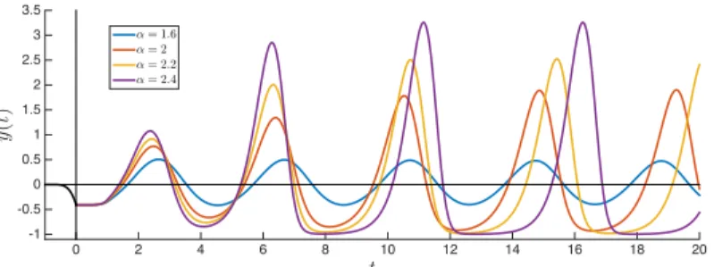
was brought to the attention of the number theorist Wright (a former Ph.D. student of Hardy at Oxford) because it arose in the application of probability methods to the theory of distribution of prime numbers. In 1955, Wright considered the more general equation (1.1) and studied the existence of bounded non trivial solutions for different values ofα >0 [13]. In 1962, following the pioneer work of Wright, Jones demonstrated in [14] that non trivial periodic solutions of (1.1) exist forα > ^π₂, and using numerical simulations, he remarked in [15] that a given periodic solution seemed to be globally attractive, that is seemed to attract all initial conditions. In Figure 3 and Figure 4, we reproduced some of the numerical simulations of Jones using the integrator for delay equationsdde23inMATLAB. The periodic form he referred to is in fact a slowly oscillating periodic solution.

t

0 2 4 6 8 10 12 14 16 18 20

y(t)

-1 -0.5 0 0.5 1 1.5 2 2.5 3 3.5 4

y0(t) =t y0(t) =−(t+ 0.8)⁴ y0(t) =t² y0(t) = 1−2|t−0.5|

Figure 3. Numerical integration of Wright’s equation (1.1) with α= 2.4 with different initial conditionsy0defined on the interval [−1,0].

t

0 2 4 6 8 10 12 14 16 18 20

y(t)

-1 -0.5 0 0.5 1 1.5 2 2.5 3 3.5

α= 1.6 α= 2 α= 2.2 α= 2.4

Figure 4. Numerical integration of Wright’s equation (1.1) with the initial condition y0(t) = −(t+ 0.8)⁴ for different parameter values ofα.

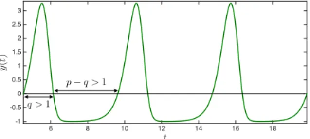
Definition 1.1. A slowly oscillating periodic solution (SOPS) of (1.1) is a periodic solutiony(t) with the following property: there exist q >1 andp > q+ 1 such that, up to a time translation, y(t) > 0 on (0, q), y(t) < 0 on (q, p), and y(t+p) =y(t)for allt so thatpis the minimal period of y(t).

A geometric interpretation of a SOPS is found in Figure 5.

After Jones observation in [15], the question of the uniqueness of SOPS in (1.1) became popular and is still under investigation after more than 50 years. The next conjecture is sometimes calledJones Conjecture.

t

6 8 10 12 14 16 18

y(t)

-1 -0.5 0 0.5 1 1.5 2 2.5 3

q >1

p q >1

Figure 5. A slowly oscillating periodic solution.

Conjecture 1.1 (Jones, 1962). For everyα > ^π₂, (1.1) has a unique SOPS.

A result of Walther in [16] shows that if Jones Conjecture is true, then the unique SOPS attracts a dense and open subset of the phase space. A result from Chow and Mallet-Paret from [17] shows that there is a supercritical Hopf bifurca- tion of SOPS from the trivial solution at α = π/2. This branch of SOPS which bifurcates (forward in α) from 0 is denoted by F⁰. We refer to Figure 6 for a geometric interpretation of bifurcation.

α

||y||

F0

π 2

Figure 6. A supercritical Hopf bifurcation of SOPS from 0 atα=π/2.

Regala then proved in his Ph.D. thesis [18] a result which implies that there cannot be any secondary bifurcations fromF⁰. Hence,F⁰is a regular curve in the (α, y) space. Later, Xie used asymptotic estimates for large α to prove that for α >5.67, Wright’s equation has a unique SOPS up to a time translation [19, 20].

Combining the strategy employed by Xie with a rigorous numerical integrator, the recent work of Jaquette et al. [21] proves that Wright’s equation has a unique SOPS for all parameter value α ∈ [1.9,6.0]. In [12], it was demonstrated, using the techniques that we introduce in the present paper, that the branchF⁰does not have a fold over the parameter range π/2 + 7.3165×10⁻⁴,2.3

. The recent work [22] shows that the branch F⁰ does not have any fold over the parameter range

π/2, π/2 + 6.83×10⁻³

. Considering the work that has been done in the last 50 years, Jones Conjecture is reformulated as follows.

Conjecture 1.2 (Jones Conjecture reformulated). There are no con- nected components (isolas) of SOPS disjoint from F⁰ over the parameter range (^π₂,1.9].

We refer to Figure 7 for a cartoon picture of a scenario which would violate Jones Conjecture.

k x k

↵

⇡/2 1.9

F

F

Figure 7. A scenario which would violate Jones Conjecture: the existence of an isola F¹ of SOPS in the parameter range α ∈ (^π₂,1.9].

Remark 1.2. Another important long standing open problem, which was re- cently settled combining the results of [22] and [23] using the tools of rigorous computing, is Wright’s conjecture, which states that for allα∈(0, π/2] the global attractor of Wright’s equation is given by the origin.

The study of Conjecture 1.2 naturally lead to study branches of periodic solu- tions of DDEs. This is the main topic of these notes. More precisely, we introduce a general continuation method to compute global branches of periodic solutions of DDEs using Fourier series and the ideas from rigorous computing (e.g. see [24]).

Note that the study of periodic solutions in DDEs is rich [25, 26, 27, 28, 29, 30, 31, 32]. Rather than focussing only on continuation of periodic solutions in DDEs, we present in Section 2 a more general approach to prove existence of branches of solutions for operator equationsF(x, λ) = 0 posed on Banach spaces. In Section??, we apply the general method to the context of periodic solutions of DDEs.

2. Rigorous Continuation of Solutions

Throughout this section, let (X,k · k^X) and (Y,k · k^Y) denote Banach spaces.

The vectors spacesXandY are general and are either finite or infinite dimensional.

LetF :X×R→Y aC¹mapping (see Definition 2.2), and consider the general problem of looking for solutions of

(2.1) F(x, λ) = 0,

where λ ∈ R is a parameter. The unknown variable x could represent various types of dynamical objects, e.g. a steady state of a PDE, a periodic solution of a DDE, a connecting orbit of an ODE, a minimizer of an action functional, etc. It is important to realize that thesolution set

S ^def= {(x, λ)∈X×R|F(x, λ) = 0} ⊂X×R

may contain different types of bifurcations and may be complicated (e.g. see Fig- ure 8).

kxk

0 0.005 0.01 0.015 0.02 0.025 0.03

0 0.05 0.1 0.15 0.2 0.25 0.3 0.35 0.4 0.45 0.5

•

• •

••

• _•

•••

• • •

•• •

••

• ^{• •}

• •

S

Figure 8. Global branches of steady states of a system of reaction-diffusion PDEs introduced in [33] and studied with rigor- ous numerics in [34].

There exists a vast literature on numerical continuation methods to compute solutions of (2.1). Methods to compute periodic orbits [35, 36], connecting orbits [37, 38, 39, 40] and more generally coherent structures [41] are by now standard, and software packages like AUTO [42] and MATCONT [43] are accessible and well documented. We refer to [44, 45] for more general references on continuation methods. Next we briefly introduce two main algorithms to compute solutions of (2.1), namely the parameter continuation and the pseudo-arclength continuation.

These methods fall into the class of predictor-corrector algorithms.

2.1. Predictor-Corrector Algorithms. In this section, we assume that the Banach spaces are finite dimensional and given by X =Y =Rⁿ (X =Y =Cⁿ is also an option), we consider a map F : Rⁿ×R → Rⁿ and we study numerically the problemF(x, λ) = 0. At this point, consideringX andY finite dimensional is natural, as any computer algorithm needs to be applied to a problem with a finite resolution. The mapping F could be a finite-dimensional projection of an infinite dimensional operator, e.g. a Galerkin approximation or a discretization scheme.

The first predictor-corrector algorithm we introduce is parameter continuation.

2.1.1. Parameter Continuation. This method involves a predictor and a cor- rector step: given, within a prescribed tolerance, a solutionx0 at parameter value λ0, the predictor step produces an approximate solution ˆx0 at nearby parameter valueλ1=λ0+ ∆λ(for some ∆λ6= 0), and the corrector step, takes ˆx1as its input and produces with Newton’s method, once again within the prescribed tolerance, a solutionx1atλ1.

The predictor is obtained by assuming that at the solution (x0, λ0), the jacobian matrix DxF(x0, λ0) is invertible, which in turns implies by the implicit function theorem that the solution curve is locally parametrized byλ. In this case, close to (x0, λ0), we have

∂

∂λ(F(x, λ) = 0)⇐⇒DxF(x, λ)dx

dλ(λ)+∂F

∂λ(x, λ) = 0⇐⇒ dx

dλ(λ) =−DxF(x, λ)⁻¹∂F

∂λ(x, λ).

1 0

S

x0

˙ x0

x1

kxk

ˆ x1

Figure 9. Parameter continuation.

At (x0, λ0), a tangent vector to the curve is ˙x0

def= ^dx_dλ(λ0) and is obtained with the formula

˙

x0=−DxF(x0, λ0)⁻¹∂F

∂λ(x0, λ0).

Once the tangent vector ˙x0is obtained, the predictor is defined by ˆ

x1=x0+ ∆λx˙0.

Then, fixingλ1=λ0+ ∆λ, wecorrectthe predictor ˆx1using Newton’s method x⁽⁰⁾₁ = ˆx1, x⁽ⁿ⁺¹⁾₁ =x⁽ⁿ⁾₁ −

DxF(x⁽ⁿ⁾₁ , λ1)−1

F(x⁽ⁿ⁾₁ , λ1), n≥0, to obtain the solution x1 at λ1 within the prescribed tolerance. We repeat this procedure iteratively to produce numerically a branch of solutions. We refer to Figure 9 to visualize one step of the parameter continuation algorithm.

Sometimes it may be more natural to parametrize the branches of solutions of (2.1) by arclength or pseudo-arclength, especially when the solution curve is not locally parametrized byλ, for instance at points where the jacobian matrix is singular. This is for instance what is happening when a saddle-node bifurcations (folds) occur. An example of such phenomenon is given byF(x, λ) =x²−λ= 0 at the point (x0, λ0) = (0,0). Pseudo-arclength continuation, as opposed to parameter continuation, allows continuing past folds.

2.1.2. Pseudo-Arclength Continuation. In the pseudo-arclength continuation algorithm (e.g. see Keller [46]), the parameter value λ is no longer fixed and instead is left as a variable. The unknown variable is nowX = (x, λ). Consider the problem F(X) = 0 with the map F :Rⁿ⁺¹ →Rⁿ. As before, the process begins with a solutionX0given within a prescribed tolerance. To produce a predictor, we compute first a unit tangent vector to the curve at X0, that we denote ˙X0, which is computed using the formula

DXF(X0) ˙X0=

DxF(¯x0,λ¯0) ∂F

∂λ(x0, λ0)

X˙0= 0∈Rⁿ. We now fix apseudo-arclength parameter∆s>0, and set the predictor to be

Xˆ1

def= ¯X0+ ∆sX˙0∈Rⁿ⁺¹.

Once the predictor is fixed, wecorrecttoward the setSon the hyperplane perpen- dicular to the tangent vector ˙X0which contains the predictor ˆX1. The equation of this plan is given by

E(X) ^def= (X−Xˆ1)·X˙0= 0.

Then, we apply Newton’s method to the new function

(2.2) X 7→

E(X) F(X)

with the initial condition ˆX1 to obtain a new solution X1 given again within a prescribed tolerance. See Figure 10 for a geometric interpretation of one step of the pseudo-arclength continuation algorithm. At each step of the algorithm, the function defined in (2.2) changes since the plane E(X) = 0 changes. With this method, it is possible to continue past folds. Repeating this procedure iteratively produces a branch of solutions.

S

kxk

X1

X0

X˙0 s Xˆ1

Figure 10. Pseudo-arclength continuation.

Remark 2.1. The above mentioned algorithms do not cover the case of bifur- cations of solutions e.g. symmetry-breaking pitchfork bifurcations, branch points, Hopf bifurcations, etc. We refer for instance to the work [44] for numerical contin- uation methods handling bifurcations.

Now that we have briefly introduced two classical algorithms to numerically compute branches of solutions of the general problem (2.1), we present an approach that combines the strength of the numerical continuation methods with the ideas of rigorous computing (e.g. see [24]). Before introducing the rigorous continuation method in Section 2.3, we need some background from calculus in general Banach spaces.

2.2. Background of Calculus in Banach Spaces. The space of bounded linear operators is defined by

B(X, Y) ^def=

E: X→Y |E is linear, kEk^B(X,Y)<∞ , wherek · kB(X,Y) denotes the operator norm

kEk^{B(X,Y) def}= sup

kxkX=1kExk^Y.

Note that B(X, Y),k · kB(X,Y)

is a Banach space.

Definition 2.2. A function F: X →Y isFr´echet differentiable atx0∈X if there exists a bounded linear operatorE:X→Y satisfying

khlimkX→0

kF(x0+h)−F(x0)−Ehk^Y khk^X = 0.

The linear operator E is called the derivative of F at x0 and denoted by E = DxF(x0). We say that F:X → Y is a C¹ mapping if for every x ∈ X, F is Fr´echet differentiable at x.

Given a point x0 ∈X and a radius r > 0, denote by Br(x0)⊂X the closed ball of radiusrcentered atx0, that is

Br(x0) ^def= {x∈X| kx−x0k^X≤r}.

The proof of the following version of the Mean Value Theorem is found in [47].

Theorem2.3 (Mean Value Theorem).Letx0∈X and suppose thatF: Br(x0)⊂ X →Y is aC¹ mapping. Let

K ^def= sup

x∈Br(x0)kDxF(x)k^B(X,Y). Then for anyx, y∈Br(x0)we have that

kF(x)−F(y)k^Y ≤Kkx−yk^X.

While the following concept could be introduced more generally in the context of metric spaces, we present it in the context of Banach spaces to best suit our needs.

Definition2.4. Suppose thatΛis a set of parameters. A functionT:X×Λ→ X is auniform contractionif there exists κ∈[0,1) such that, for allx, y∈X and λ∈Λ,

kT(x, λ)−T(y, λ)k^X ≤κkx−yk^X.

By the Contraction Mapping Theorem if T: X ×Λ → X is a uniform con- traction, then for every λ∈Λ there exists a unique ˜xλ such that T(˜xλ, λ) = ˜xλ. Thus the functiong: Λ→X given byg(λ) ^def= ˜xλis well defined. As the following theorem indicates this function inherits the same amount of differentiability than T. The proof is found in [47].

Theorem 2.5 (Uniform Contraction Theorem). Assume that the set of parameters Λ is a Banach space, and consider open sets U ⊂ X and V ⊂ Λ.

Assume thatT:U×V →U is a uniform contraction with contraction constant κ.

Define g:V →U byT(g(λ), λ) = g(λ). IfT ∈C^k(U×V, X), then g ∈C^k(V, X) for any k∈ {1,2, . . . ,∞}.

2.3. The Rigorous Continuation Method. Now that we have introduced some basic notions from calculus in Banach spaces, we are ready to present the gen- eral rigorous continuation method. The idea of the proposed approach is to prove the existence of true solution segments of F(x, λ) = 0 close to piecewise-linear segments of approximations by applying the Uniform Contraction Theorem (The- orem 2.5) over intervals of parameters. This approach has the advantage of being quite general and is readily generalized to problems depending of several parameters (e.g. see Remark 2.9). However, the rigorous error bounds quickly deteriorate as

the width of the interval of parameters (on which the uniform contraction theorem is applied) grows. This is due to the fact that piecewise-linear approximations are coarse approximations of the solution branches of nonlinear problems. Expanding the solutions using high order Taylor approximations in the parameter could for instance increase significantly the error bounds (e.g. see [48, 49]), at the cost of complicating the analysis. This being said, let us mention the existence of a grow- ing literature on rigorous numerical methods to compute branches of parameterized families of solutions [34, 50, 51, 52, 53].

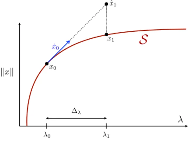
Assume that numerical approximations of (2.1) have been obtained at two different parameter valuesλ0andλ1, namely there exists (¯x0, λ0) and (¯x1, λ1) such that F(¯x0, λ0) ≈ 0 and F(¯x1, λ1) ≈ 0. In other words, (¯x0, λ0) and (¯x1, λ1) are approximately in the solution set S (e.g. see Figure 11). The approximations are computed first by considering a finite dimensional projection of F and then by using one of the two predictor-correctors algorithms presented in Section 2.1. We refer to Section 2.5.3 for an example in the context of periodic solutions of DDEs.

Define the set ofpredictors between the approximations (¯x0, λ0) and (¯x1, λ1) by (2.3) {(¯xs, λs)|x¯s= (1−s)¯x0+s¯x1 and λs= (1−s)λ0+sλ1, s∈[0,1]}.

1 0

¯ x1

¯ x0

S

¯ xs

kxk r

Figure 11. The set of predictors {(¯xs, λs)|s∈[0,1]}, approxi- mating a segment of the solution set S. The radii polynomial approach, when successful, provides a “tube” of with r >0 (the shaded region ) inX×R, where the true segment of solution curve is guaranteed to exist.

Consider bounded linear operatorsA^†∈B(X, Y) andA∈B(Y, X), whereA^†is an approximation ofDxF(¯x0, λ0) andAis an approximate inverse ofDxF(¯x0, λ0).

Assume thatAis injective and that

(2.4) AF:X×R→X.

The following theorem, often called the radii polynomial approach, is a pa- rameter dependent Newton-Kantorovich theorem (e.g. see [54]) with a smoothing approximate inverse.

Theorem 2.6 (Radii Polynomial Approach). Assume that F ∈ C^k(X× R, Y) withk∈ {1,2, . . . ,∞}, and letY0, Z0, Z1, Z2≥0 satisfying

kAF(¯xs, λs)k^X ≤Y0, ∀s∈[0,1]

(2.5)

kI−AA^†kB(X,X)≤Z0

(2.6)

kA[DxF(¯x0, λ0)−A^†]k^B(X,X)≤Z1

(2.7)

kA[DxF(¯xs+b, λs)−DxF(¯x0, λ0)]kB(X,X)≤Z2(r), ∀ b∈Br(0) and∀s∈[0,1].

(2.8)

Define the radii polynomial

(2.9) p(r) ^def= Z2(r)r+ (Z1+Z0−1)r+Y0. If there exists r0>0 such that

p(r0)<0, then there exists aC^k function

˜

x: [0,1]→ [

s∈[0,1]

Br₀(¯xs) such that

F(˜x(s), λs) = 0, ∀ s∈[0,1].

Furthermore, these are the only solutions in thetube S

s∈[0,1]Br0(¯xs).

Proof. Recalling (2.4), define the operatorT:X×[0,1]→X by T(x, s) =x−AF(x, λs).

We begin by showing that for eachs∈[0,1], the operatorT(·, s) is a contraction mapping fromBr0(¯xs) into itself. Now, giveny∈Br0(¯xs) and applying the bounds (2.5), (2.6), (2.7), and (2.8), we obtain

kDxT(y, s)kB(X,X)=kI−ADxF(y, λs)kB(X,X)

≤ kI−AA^†k^B(X,X)+kA[DxF(¯x0, λ0)−A^†]k^B(X,X) +kA[DxF(y, λs)−DxF(¯x0, λ0)]kB(X,X)

≤Z0+Z1+Z2(r0).

(2.10)

We now show that for eachs∈[0,1] the operatorT(·, s) maps Br0(¯xs) into itself.

Lety∈Br0(¯xs) and apply the Mean Value Theorem (Theorem 2.3) to obtain kT(y, s)−x¯sk^X ≤ kT(y, s)−T(¯xs, s)k^X+kT(¯xs, s)−x¯sk^X

≤ sup

b∈Br0(¯xs)kDxT(b, s)k^B(X,X)ky−x¯sk^X+kAF(¯xs, λs)k^X

≤(Z0+Z1+Z2(r0))r0+Y0

where the last inequality follows from (2.10). Recalling (2.9) and using the assump- tion that p(r0)<0 implies thatkT(y, s)−x¯sk^X < r0 for alls∈[0,1], the desired result.

Lettinga, b∈Br0(¯xs), apply the Mean Value Theorem and (2.10) to obtain kT(a, s)−T(b, s)k^X ≤ sup

b∈B_r0(¯x_s)kDxT(b, s)kB(X,X)ka−bk^X

≤(Z0+Z1+Z2r0)ka−bk^X. (2.11)

Again, from the assumption thatp(r0)<0, it follows fromY0≥0 that (2.12) κ ^def= Z0+Z1+Z2(r0)<1−Y0

r0 ≤1.

Define the operator

Te:Br0(0)×[0,1]→Br0(0)

(y, s)7→T(y, s)e ^def= T(y+ ¯xs, s)−x¯s.

Consider nowx, y∈Br0(0) ands∈[0,1]. Then, sincex+ ¯xs, y+ ¯xs∈Br0(¯xs), we use (2.11) and (2.12) to get

kTe(x, s)−Te(y, s)k^X =kT(x+ ¯xs, s)−T(y+ ¯xs, s)k^X

≤κkx−yk^X.

Sinceκ <1, we conclude thatTe:Br0(0)×[0,1]→Br0(0) is a uniform contraction.

By the Uniform Contraction Theorem (Theorem 2.5), there existsg: [0,1]→Br0(0) by

T(g(s), s) =e g(s).

Since F ∈C^k(X×R, Y), thenTe∈ C^k(Br0(0)×[0,1], Br0(0)), and therefore g ∈ C^k([0,1], Br0(0)). Let

˜

x(s) ^def= g(s) + ¯xs

so that for alls∈[0,1]

T(˜x(s), s) =T(g(s) + ¯xs, s) =Te(g(s), s) + ¯xs=g(s) + ¯xs= ˜x(s).

SinceT(x, s) =x−AF(x, λs), we get that

T(˜x(s), s) = ˜x(s)−AF(˜x(s), λs) = ˜x(s).

By assumption thatAis injective,

F(˜x(s), λs) = 0, ∀ s∈[0,1].

It follows fromg∈C^k([0,1], Br0(0)) that

˜

x: [0,1]→ [

s∈[0,1]

Br0(¯xs)

is a C^k function. Furthermore, it follows from the contraction mapping theorem that these are the only solutions in thetubeS

s∈[0,1]Br0(¯xs)×[λ0, λ1].

Theorem 2.6 provides a recipe to compute a local segment of solution curve and to obtain a uniform rigorous error boundr along the set of predictors connecting two numerical approximations ¯x0 and ¯x1. See Figure 11 for a representation of the region (shaded) where the true segment of solution curve is guaranteed to exist. Assume now that this argument has been repeated iteratively over the set {x¯0, . . . ,x¯j} of approximations at the parameter values {λ0, . . . , λj} respectively.

For each i = 0, . . . , j−1, this yields the existence of a unique portion of smooth solution curveSⁱ in a smalltubecentered at the segment {(1−s)¯xi+s¯xi+1 |s∈ [0,1]}. As the following results demonstrates, the set

S ^def=

j−1

[

i=0

Sⁱ is a global smooth solution curve ofF(x, λ) = 0.

Lemma 2.7 (Globalizing the C^k solution branch). Assume that the radii polynomial approach was successfully applied (via Theorem 2.6) to show the exis- tence of two C^k segments S0 and S1 of solution curves parameterized by the pa- rameterλover the respective parameter intervals[λ0, λ1]and[λ1, λ2]. Assume that the sets of predictors are defined by the three points x¯0,x¯1 and ¯x2. Then the new segment of solution curveS0∪S1 is aC^k function of λ.

Proof. The continuity ofS0∪S1follows from the fact that at the parameter valueλ=λ1, the solution segmentS0must connect continuously with the solution segmentS1 by the existence and uniqueness result guaranteed by the Contraction Mapping Theorem. Letp0(r) the radii polynomial built with the predictors gener- ated by ¯x0and ¯x1, and defined by the boundsY0, Z0, Z1 andZ2. Letr0>0 such that p0(r0)<0. By continuity of the radii polynomialp0, there exists δ0 >0 and there exist bounds ˜Y0(δ0) and ˜Z2(r, δ0) such that

kAF(¯xs, λs)k^X ≤Y˜0(δ0), ∀ s∈[−δ0,1 +δ0]

kA[DxF(¯xs+b, λs)−DxF(¯x0, λ0)]kB(X,X)≤Z˜2(r, δ0), ∀b∈Br(0), ∀s∈[−δ0,1 +δ0], and such that

˜

p0(r0) ^def= ˜Z2(r0, δ0)r0+ (Z1+Z0−1)r0+ ˜Y0(δ0)<0.

Then, there exists of a C^k branch of solution curve parameterized by λover the range{(1−s)λ0+sλ1|s∈[−δ0,1 +δ0], extending smoothly (in fact in aC^k way) the segmentS0 on both sides. Similarly, there existsδ1 such that the segmentS1

is extended smoothly over the parameter range{(1−s)λ1+sλ2|s∈[−δ0,1 +δ0].

This implies that there is aC^k overlap betweenS0 andS1.

•

• _•

¯

x

x ¯

x ¯

k x k

2 1

0

S

S

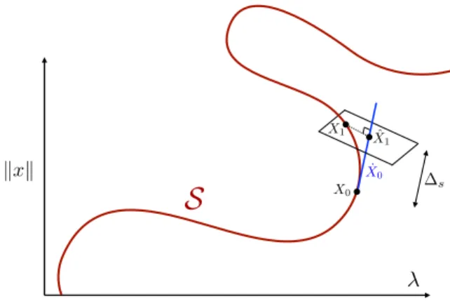
Figure 12. Assume thatS0 andS1 are computed with the radii polynomial approach with predictors defined by three points ¯x0,

¯

x1 and ¯x2 with ¯xi ∈C^2m for some fixed dimension m. Then the following situation is not possible: a piecewise smooth but not globally smooth piece of solution curve.

Note that arguments using the continuity of the radii polynomials, as in the proof of Lemma 2.7, are not new and have been used previously in the works [34, 52, 53].

Repeating iteratively the argument of Lemma 2.7 leads to the existence of a smooth solution curveSofF = 0 near the piecewise linear curve of approximations, as portrayed in Figure 13.

•

•

•

•

• _• •

¯ x

¯ x

¯ x

¯ x

¯ x

¯ x

¯ x

¯ x

• k x k

S

j 1

j 2 j

4 2 3

1 0

Figure 13. Computing rigorously a global branch of solutions.

Remark 2.8 (Bifurcations). In the present work we do not discuss how to handle some type bifurcations. Instead, we refer to the paper of Thomas Wanner [55], where a rigorous computational method to prove existence of saddle-node bifurcations and symmetry-breaking pitchfork bifurcations is presented.

Remark 2.9 (Number of Parameters and Multi-parameter Continua- tion). In the present work, we focus on equations depending on a single parameter λ ∈ R. However, the radii polynomial approach (as presented below in Theo- rem 2.6) works also for problems depending on p > 1 parameters. In fact, the method may be extended to prove existence of “solution manifolds” within solu- tions sets of the form{(x,Λ)∈X×R^p|F(x,Λ) = 0}. The only difference is that the bounds which need to be computed to apply the uniform contraction theorem have to be obtained uniformly over a compact set of parameters inR^pinstead of in R. A more advanced approach based on a rigorous multi-parameter continuation method, generalizing the concept of pseudo-arclength continuation, is introduced in [53] to compute solutions manifolds and to handle higher dimensional folds.

Remark 2.10 (Parameter Continuation vs Pseudo-Arclength Contin- uation). The method of Theorem 2.6 is based on parameter continuation: we compute branches of solutions parametrized by the parameter λ. The method is extended to pseudo-arclength continuation where solutions are parametrized by pseudo-arclength (e.g. see [52, 34]).

Remark 2.11 (Computing the boundY0). To compute theY0 bound sat- isfying (2.5), denote

∆¯x ^def= ¯x1−x¯0 and ∆λ ^def= λ1−λ0, and consider the expansion

F(¯xs, λs) =F(¯x0, λ0) +

DxF(¯x0, λ0) ∂F

∂λ(¯x0, λ0) ∆¯x

∆λ

s +1

2 ∂²

∂s²F(¯xs, λs) s=0

s²+h.o.t.

Denote

y1 def=

DxF(¯x0, λ0) ∂F

∂λ(¯x0, λ0) ∆¯x

∆λ (2.13)

y2 def= 1

2 ∂²

∂s²F(¯xs, λs) s=0

. (2.14)

Hence,

kAF(¯xs, λs)k^X≤ kAF(¯x0, λ0)k^X+kAy1k^X+kAy2k^X+δ where the extra termδ≥0 is obtained using Taylor remainder’s theorem.

2.4. A Finite Dimensional Example. In this section, we apply the radii polynomial approach (Theorem 2.6) to prove the existence of branches of solutions of the problem (2.1) withF a mapping between finite dimensional Banach spaces.

The example we consider is the problem of computing branches of steady states for the atmospheric circulation model introduced by Edward N. Lorenz in [56]

(2.15)







x⁰₁=−αx1−x²₂−x²₃+αλ x⁰₂=−x2+x1x2−βx1x3+γ x⁰₃=−x3+βx1x2+x1x3.

Let us fix α = 0.25, β = 4 and γ = 0.5, and leave λ as a parameter. At these parameter values, equilibria of (2.15) are solutions of

(2.16) F(x, λ) ^def=





−¹4x1−x²₂−x²₃+^λ₄

−x2+x1x2−4x1x3+¹₂

−x3+ 4x1x2+x1x3



= 0.

In this case, the Banach spaces areX =Y =R³endowed with the sup-norm kxk= max(|x1|,|x2|,|x3|).

Atλ0= 0.8 and λ1= 0.85, we used Newton’s method to compute respectively

¯ x0=





−0.056551859183890 0.452495729654079

−0.096879200248534



 and x¯1=





−0.043505480122129 0.466188932513298

−0.077744769808933



.

We wish to use Theorem 2.6 to prove the existence of a segment of solutions in the solution set S = {(x, λ)∈ R⁴ | F(x, λ) = 0}. For s∈ [0,1], recall the set of predictors (2.3) given by ¯xs= (1−s)¯x0+s¯x1and letλs= (1−s)λ0+sλ1. Denote by

∆¯x ^def= ¯x1−x¯0 and ∆λ ^def= λ1−λ0.

Recalling the Y0 bound satisfying (2.5). Since the vector field is quadratic, recalling (2.13) and (2.14), we get the following expansion

F(¯xs, λs) =F(¯x0, λ0) +y1s+y2s², where

y2=





−(∆¯x)²₂−(∆¯x)²₃ (∆¯x)1(∆¯x)2−4(∆¯x)1(∆¯x)3

4(∆¯x)1(∆¯x)2+ (∆¯x)1(∆¯x)3



.

The matrixA≈DF(¯x0, λ0)⁻¹ is computed usingMATLABand is given by A=





−1.031444307007117 0.883485538811585 0

−1.126473748855484 0.059891724595854 −0.193758400497068

−1.431216390563831 1.419669460728974 −0.904991459308157



.

Using the definition of A, y1 and y2, we computeY0 = 0.002488451115105. For this finite dimensional example, we setA^† =DF(¯x0, λ0), so thatZ1 = 0 in (2.7).

Recalling (2.6), we set Z0 = kI−ADF(¯x0, λ0)k∞. In this case, we computed Z0 = 2.27×10⁻¹⁶. To facilitate the computation of Z2 satisfying (2.8), consider c∈B1(0)⊂R³, that iskck∞≤1, and consider b∈Br(0)⊂R³, that iskbk∞≤r.

Then,

[DxF(¯xs+b, λs)−DxF(¯x0, λ0)]c=





−2b2c2−2b3c3

b1c2−4b1c3+b2c1−4b3c1

4b1c2+b1c3+ 4b2c1+b3c1





+s





−2c2(∆¯x)2−2c3(∆¯x)3

c1(∆¯x)2−4c1(∆¯x)3+c2(∆¯x)1−4c3(∆¯x)1

4c1(∆¯x)2+c1(∆¯x)3+ 4c2(∆¯x)1+c3(∆¯x)1



,

and since|s| ≤1, we get the component-wise inequalities

|[DxF(¯xs+b, λs)−DxF(¯x0, λ0)]c| ≤



 4 10 10



r+





2|(∆¯x)2|+ 2|(∆¯x)3|

|(∆¯x)2|+ 4|(∆¯x)3|+ 5|(∆¯x)1| 4|(∆¯x)2|+|(∆¯x)3|+ 5|(∆¯x)1|



.

Hence, letting Z₂^{(1) def}=

|A|



 4 10 10



 ∞

and Z₂^{(0) def}=

|A|





2|(∆¯x)2|+ 2|(∆¯x)3|

|(∆¯x)2|+ 4|(∆¯x)3|+ 5|(∆¯x)1| 4|(∆¯x)2|+|(∆¯x)3|+ 5|(∆¯x)1|



 ∞

we set

Z2(r) =Z₂⁽¹⁾r+Z₂⁽⁰⁾.

Numerically, we obtainZ₂⁽¹⁾= 28.971474762626638 andZ₂⁽⁰⁾= 0.440592442217924.

Recalling (2.9) and thatZ1= 0, the radii polynomial is given by p(r) =Z2(r)r+ (Z0−1)r+Y0

=Z₂⁽¹⁾r²+ (Z₂⁽⁰⁾+Z0−1)r+Y0

= 28.971474762626638r²−0.559407557782076r+ 0.002488451115105.

Note that

I ^def= {r >0|p(r)<0} ⊃[0.006949765480451, 0.012359143105166].

Choosing for instance r0 = 0.007 ∈ I, then by Theorem 2.6, there exists a C^∞ function

˜

x: [0,1]→ [

s∈[0,1]

Br0(¯xs)

such thatF(˜x(s), λs) = 0 for alls∈[0,1] withF given in (2.16), and these are the only solutions in the setS

s∈[0,1]Br0(¯xs)×[λ0, λ1].

Also, we applied the method on the intervals of parameters [λ1, λ2] and [λ2, λ3] corresponding respectively to the segments{(1−s)¯x1+s¯x2|s∈[0,1]}and{(1− s)¯x2+s¯x3|s∈[0,1]}, withλ2= 0.89,λ3= 0.925, and

¯ x2=





−0.032746172312211 0.476481288735590

−0.060432810317938



 and x¯3=





−0.022963874112357 0.484866398590268

−0.043537846136356



.

The MATLAB program script proof lorenz.m available at [76] performs the above computations. It uses the interval arithmetic packageINTLAB devel- oped by Siegfried M. Rump [57].

λ

0.8248 0.8248 0.8249 0.8249 0.8250 0.825 0.8251 0.8251

x

-0.0504 -0.0503 -0.0502 -0.0501 -0.05 -0.0499 -0.0498

λ

0.5 0.6 0.7 0.8 0.9 1 1.1 1.2

x

0 0.2 0.4 0.6 0.8 1

Figure 14. (Left) A branch of equilibria for the model (2.15) computed using the pseudo-arclength continuation algorithm as presented in Section 2.1.2. The segments in red, green and pur- ple were rigorously computed with the radii polynomial approach.

The respective error bounds between the predictors and the actual solution segments arer0= 7×10⁻³(red),r0= 4.2×10⁻³ (green) andr0 = 3.9×10⁻³ (purple). (Right)A zoom-in on the branch where the proof was performed atλ= 0.825.

Remark 2.12 (Proofs at fixed parameter values). It is important to re- call that the purpose of the present section is to introduce a method to com- pute “branches” of solutions. If however we are interested in proving the ex- istence of a solution at a fixed parameter value, then we get dramatically bet- ter error bounds. Let us do this exercise for model (2.15) with the approxima- tion ¯x0. In this case, ∆¯x = 0 ∈ R³, ∆λ = 0 and Z₂⁽⁰⁾ = 0, the radii poly- nomial is p(r) = 28.971474762626652r² + (2.195852227948092×10⁻¹⁵ −1)r+ 2.449129914171945×10⁻¹⁶, and

I ^def= {r >0|p(r)<0} ⊃

2.45×10⁻¹⁶ , 0.034516710253563 .

0 0.005 0.01 0.015

×10^-3

0 0.5 1 1.5 2 2.5

Y0

I

r p(r)

Figure 15. The radii polynomial p(r) =Z₂⁽¹⁾r²+ (Z₂⁽⁰⁾+Z0− 1)r+Y0 associated to the numerical approximations ¯x0 and ¯x1 as defined above.

Therefore, there exists a unique ˜x0 ∈B2.45×10⁻¹⁶(¯x0) such thatF(˜x0, λ0) = 0. In this case, the rigorous error bound is of the order of 10⁻¹⁶, as opposed to 10⁻³ for the branch of solutions.

0 0.005 0.01 0.015 0.02 0.025 0.03

×10^-3

-8 -7 -6 -5 -4 -3 -2 -1 0

I

r

Figure 16. The radii polynomialp(r) =Z₂⁽¹⁾r²+ (Z0−1)r+Y0

associated to the single numerical approximation ¯x0.

We are now ready to present the main application of the rigorous continuation method.

In this section, we show how the radii polynomial approach (Theorem 2.6) is used to compute rigorously branches of periodic solutions of DDEs. Rather than presenting the ideas for general classes of problems, we focus on presenting the ideas for specific examples, namely for a delayed Van der Pol equation and for Wright’s equation. For the delayed Van der Pol equation, we present in details in Section 2.5 all steps, bounds, necessary estimates, choices of function spaces and the explicit coefficients of the radii polynomial, whereas in the case of Wright’s equation, we

only briefly discuss some results in Section 2.6 and refer to [12] for more details.

Note that the ideas presented here should be applicable to systems of N delay equations of the form

(2.17)

y⁽ⁿ⁾(t) =F

y(t), y(t−τ1), . . . , y(t−τd), . . . , y⁽ⁿ⁻¹⁾(t−τ1), . . . , y⁽ⁿ⁻¹⁾(t−τd) , wherey:R→R^N andF:R^N(nd+1)→R^N is a multivariate polynomial.

As already mentioned in Section 1 studying rigorously solutions of DDEs is a challenging problem, especially because they are naturally defined on infinite di- mensional function spaces. On the other hand, as already mentioned in Section 1, for continuous dynamical systems like (2.17), individual solutions which exist glob- ally in time are more regular than the typical functions of the natural phase space.

That suggests that solving for the Fourier coefficients of the periodic solutions of (2.17) in a Banach space of fast decaying sequences is a good strategy. In fact periodic solutions of (2.17) are analytic sinceF is analytic (it is polynomial) [10].

We therefore apriori know that the Fourier coefficients of the periodic solutions decay geometrically by the Paley-Wiener Theorem. Before presenting the rigorous numerical method, we briefly describe different methods used to study periodic solutions of (2.17), following closely the discussion in [58].

Fixed point theory, the fixed point index and global bifurcation theorems are powerful tools to study the existence of solutions of infinite dimensional dynamical systems. To give a few examples in the context of DDEs, the ejective fixed point theorem of Browder [59] and the fixed point index are used to prove existence of nontrivial periodic solutions [14, 60, 61], and the global bifurcation theorem of Rabinowitz [62] are used to prove the existence and characterize the (non) compact- ness of global branches of periodic solutions [63, 64]. This heavy machinery from functional analysis provides powerful existence results about solutions of DDEs, but its applicability may decrease if one asks more specific questions about the solutions of a given equation. For example, it appears difficult in general to use the ejective fixed point theorem to quantify the number of periodic solutions or to use a global bifurcation theorem to conclude about existence of folds, or more generally, of secondary bifurcations. The following Figure 17 taken from [32] shows that global branches of periodic solutions of DDEs may be complicated, as various bifurcations may occur on the branches. These remarks further motivate the need for rigorous numerical methods for DDEs.

Remark2.13. Let us mention the existence of other rigorous numerical meth- ods to study periodic orbits of DDEs. First, the work [65] provides a method to compute periodic solutions using a Newton-like operator and piecewise linear approximations. Second the work [66] presents a rigorous numerical integrator to prove existence of periodic orbits in the Mackey-Glass equation. Finally, let us mention that the work [67] on the parameterization method could eventually be combined with rigorous numerics to compute invariant manifolds attached to equilibria and periodic orbits.

2.5. A Delayed Van der Pol Equation. In the 1920s, the Dutch electrical engineer and physicist Van der Pol proposed his famous Van der Pol equationsto model oscillations of some electric circuits [68]. Since then, variants of the so-called

CONTINUATION OF SOLUTIONS AND STUDYING DELAY DIFFERENTIAL EQUATIONS VIA RIGOROUS NUMERICS21 then x(t; ~, ~) is a solution of equation (1.1)~ with minimal period p satisfying

(2.1o)

(2.~) and (2.1~)

1 1

Im-~l < p < Im § 89 if m < o , p > 2 if r e = O ,

1 1

m - ~ 8 9 < p < - m if m > 0 .

The sets 2/,~ are pairwise disjoint. I / m > 0 and ~ > ~,,, then equation (1.1);. has at least m + 1 distinct periodic solutions~ while i / m < 0 and A < )~, then it has at least

Im[ periodic solutions.

PROOF. - The first p a r t of the theorem h~s already been proved. The bounds (2.10)~ (2.11)~ ~nd (2.12) on the minimal period p follow immediately from the formula p ~ ~t(A, ~)/Im~(A, ~) § 1I noted above, ~nd the fact t h s t ~(A~ ~) > 2 for ()., ~s)e 2/0. These bounds also imply t h a t the sets Z~ are pairwise disjoint: one can easily check thgt the intervals of values p given in (2.10), (2.11), ~nd (2.12) for various integers m are pairwise disjoint. Finally, the connectedness, nnboundedncss and disjointness of the 2/~, the bounds (2.7), (2.8), and (2.9) for (X, ~ ) e 2 / ~ , and the ordering

... < ~ ~ < i _ ~ < 0 < A o < A ~ < )~< ...

imply the last sentence in the statement of the theorem. []

Figure 6 depicts schematically the branches X~.

li~lI

Z1

20 A 2~

Fig. 6. The global Hopf branches 2:,~.

Figure 17. Global branches of periodic solutions of delay differ- ential equations. The picture is taken directly from [32].

van der Pol oscillator have been proposed as mathematical models of various real- world processes exhibiting limit cycles when the rate of change of the state variables depend only on their current states. However, there are many processes where this relation is also influenced by past values of the system in question. To model these processes, one may want to consider the use of functional differential equations, see [9, 69, 70].

In [71], Grafton establishes existence of periodic solutions to

¨

y(t)−εy(t)(1˙ −y²(t)) +y(t−τ) = 0, ε, τ >0,

a Van der Pol equation with a retarded position variable. His results are based on his periodicity results developed in [72]. In [73], using slightly different notations, Roger Nussbaum considered the more general class of equations

(2.18) y(t)¨ −εy(t)(1˙ −y²(t)) +y(t−τ)−λy(t) = 0, ε, τ >0, λ∈R, and establishes existence of periodic solution of period greater than 2τ, given that λ∈(−λ0,1), where

λ0= min ε

τ, 2 τ²

.

We refer to (2.18) as Nussbaum’s equation. The techniques that Nussbaum uses are sophisticated fixed point arguments, however, as he remarks, he has to restrict the size of|λ| to guarantee that the zeros ofy are at least a distanceτ apart (e.g.

see p. 287 of [73]). Moreover, he mentions that numerical simulations suggest the existence of periodic solutions to (2.18) for a large range ofλ <0.

What we present now is an application of the rigorous continuation method introduced in Section 2, and we establish existence results for periodic solutions to (2.18) for parameter values outside of the range of parameters accessible with the above results of Nussbaum. The first step is to recast periodic solutions of (2.18) as solutions ofF(x, λ) = 0.

2.5.1. Setting up the F(x, λ) = 0problem. Assume thaty(t) is a periodic solu- tion of (2.18) of periodp >0. Then

(2.19) y(t) =

∞

X

k=−∞

ake^ikωt,