1
THE DETERMINANTS OF SUCCESS IN PRIMARY EDUCATION IN SPAIN
Brindusa Anghel and Antonio Cabrales March, 2010
Abstract: This study reviews the recent literature on the economics of education, with a special focus on policy interventions. It also attempts to uncover the importance of school inputs, social environment and parental background on the outcomes of a standardized exam for all sixth grade students in the region of Madrid. We have data from all exam results from 2006 to 2009. These data can then be linked to individual level characteristics such as nationality, family type and parental education and profession. For public schools we also have school level data on variables such as number of students, teachers and their characteristics (type of contracts, experience), students’ nationalities, extra-curricular activities, and number of students needing special assistance.
Keywords: Education, Human capital, Standardized tests JEL Classification: I20, I21, I28
2
1. INTRODUCTION
The productivity of an economy depends in a crucial way on the quantity and quality of the human capital accumulated by the labor force which that economy can access.
Although human capital can be in part “imported” by allowing sizable immigration flows, as Spain did in the last decade, most of it will necessarily be “home-grown.” Thus, the education system, which is a crucial piece of the human capital accumulation technology, is an essential determinant of the productivity of any economy. Furthermore, education is also important to achieve the right allocation of talent to the productive system, and hence of social mobility.
The aim of this paper is to contribute to the debate on education in Spain in a more scientific, less partisan way than what is currently available on the mass media and policy arena. The contribution is twofold. On the one hand we will review the current advances in the economic literature dealing with the different factors that affect the educational outcomes of the individuals. We will make particular emphasis on policy evaluations.
In addition to reviewing the international evidence, we take advantage of a database arising from a standardized exam that the Comunidad Autónoma de Madrid (Madrid regional government) has been conducting since 2005 for all 6th grade students in the region, who are hence in the final year of primary school. The exam measures what the authorities considers basic skills (Competencias y Destrezas Indispensables, or C.D.I.) in mathematics, language, dictation, reading and general knowledge. The exam does not have academic consequences for the children. Like the tests conducted by the PISA program, the C.D.I. exam serves mostly an informative purpose, both for the student and for the authorities.
For three years (2006, 2007, 2008) the exam grades could be linked to very few individual characteristics of the children (like gender or nationality), but we were able to obtain a good number of school-level controls (for public schools).1 For the last year (2009) we can include additional individual-level controls: the most important ones are the parents’ level of education and their profession. We will focus our empirical analysis on the data for the 2009 cohort and we will present the results for the 2006-2008 cohorts as a robustness check.
There are several conclusions one can draw both from the literature review and our data. A first consideration is that we need more evidence, as the existing one does not allow us to make very sharp predictions on the effects of many policies. In spite of that, we think that there are several recommendations which are well grounded: we need more incentives for all actors in this drama (teachers, principals, students and parents), more competition between
1Data for 2005 are available as well, but we decided not to use them, since there were no individual characteristics of the children.
3
schools and more high quality early intervention for the students in the worst socioeconomic conditions.
Why do we need more data? The availability of large longitudinal databases, such as the one we employ in this paper, has allowed us to understand many things about the education production function. But it has evident limitations. For example, it is difficult to see whether children in private schools obtain better results because the schools themselves are better, or because better performing students self-select into those schools.
The availability of enough control variables in the databases and the use of clever econometric techniques go part of the way to address this issue. But it is a partial answer to the problem, at best. Increasingly, and especially in the United States, randomized testing of different policy instruments is used to provide robust answers to questions of policy effects.
The methodological advantages of randomization are obvious, given the endogeneity problems we just mentioned. There is also a clear practical advantage. It is far cheaper to introduce a policy in a limited test-trial form, than to do a wholesale reform only to reverse it a few years later. Indeed, many educational reforms in Spain were introduced in a gradual form.
The E.S.O. (Compulsory Secondary Education) was implemented first in some schools and only in later years in the rest. Unfortunately, this was not done in a controlled way so as to make it possible to evaluate its impact. That was a great opportunity missed.
From the literature review we can see that there are no easy shortcuts. Cutting class sizes is simple to implement, but it is controversial whether it improves outcomes very much, and it is definitely very expensive. Putting more computers in the classroom is also easy, but it appears to have no discernible effect on anything other than, you guessed it, computer literacy.
Voucher schemes have contradicting effects on educational outcomes (large in some studies, smaller in others) and a likely large effect on social segregation, if they are used indiscriminately. Clearly, we need to study this policy better. And, in any case, we should concentrate its application on at-risk populations. Vouchers may also provide incentives to public schools, but they would need to be harmed by the competition directly, and be given more organizational freedom to react.
On the other hand, paying teachers, and even students, for performance definitely works. With teachers, one needs to be careful with the measure of performance, to avoid paying teachers for the luck of having already good students. In this respect, it would be useful to have better measures of value added. The difference between grades from C.D.I. exams at the end of primary and the end of compulsory secondary (E.S.O.) education could give a good measure of value added, but authorities would need to make sure the same students are evaluated. This is impossible in the current regime where the students’ results are completely
4
anonymous, since one cannot measure the difference in their performance from one exam to the next.
There are other interesting measures that would benefit from closer examination by our authorities. Grouping students by their ability has been proved to work, if the teachers are then allowed to tailor their teaching to the students’ level. Also, intensive early educational (and social) attention has also proved to yield high social returns, and is probably an important policy to undertake in the future.
With respect to our study of the Madrid data, there are several important findings to be noted. First, we summarize briefly the effects of personal characteristics, which are only available for the 2009 data. Parental education and profession are extremely important, confirming results from earlier studies. From these two factors, education is clearly more important than profession, but the two have significant independent impact. Children living with single parents do worse than the rest, and having brothers and sisters tends to be associated with good performance.
Immigrants sometimes do worse than nationals, even after controlling for parental education, but this is far from universal. Some of this is expected, as Asians or Eastern Europeans tend to do very well in mathematics and less well in language (in fact, poorly, in the case of Asians). But some of this is surprising. Moroccan students are no different from Spaniards in mathematics and general knowledge, once parental background is controlled for, although a bit worse in language and dictation. Latin Americans are the large group with the worst outcomes, even after taking into account parental background. They do worse than Spaniards in all subjects. For example, their Spanish scores are at the level of those for East Asians.
In terms of school level variables the first conclusion is that the class size2 appears to have no significant impact on students’ achievement.3 This is important because the usual response by some sectors to educational problems is: more resources are needed. The evidence on class size implies that extra resources can be easily misspent on unproductive policies.
Another useful result is that the percentage of immigrants in the class has at best a small effect on the performance of other children, and it is not statistically significant in most of the regressions At worst, we find that in dictation schools that have between 21% and 30%
immigrants in the 6th grade perform slightly better than schools that have more than 40%
immigrants in the 6th grade.
2For this variable we only have data for public schools.
3In addition to OLS, we also control for the endogeneity of class size, à la Angrist and Lavy (1999).
5
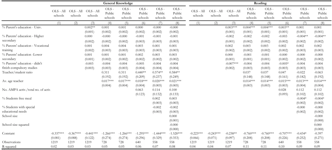
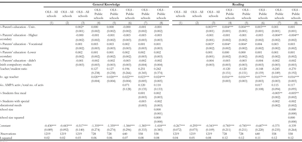
We also find that the average parental education in the class has a statistically significant impact on the school fixed effect. That is, beyond the effect of their own parental background, the children experience an additional effect coming from their peers’ parental background. This could explain why the unconditional means of schools with large amounts of immigrants are lower, even though the proportion of immigrants has no explanatory power for the fixed effect. Those badly performing schools with lots of immigrants also concentrate large amounts of children with less educated parents.
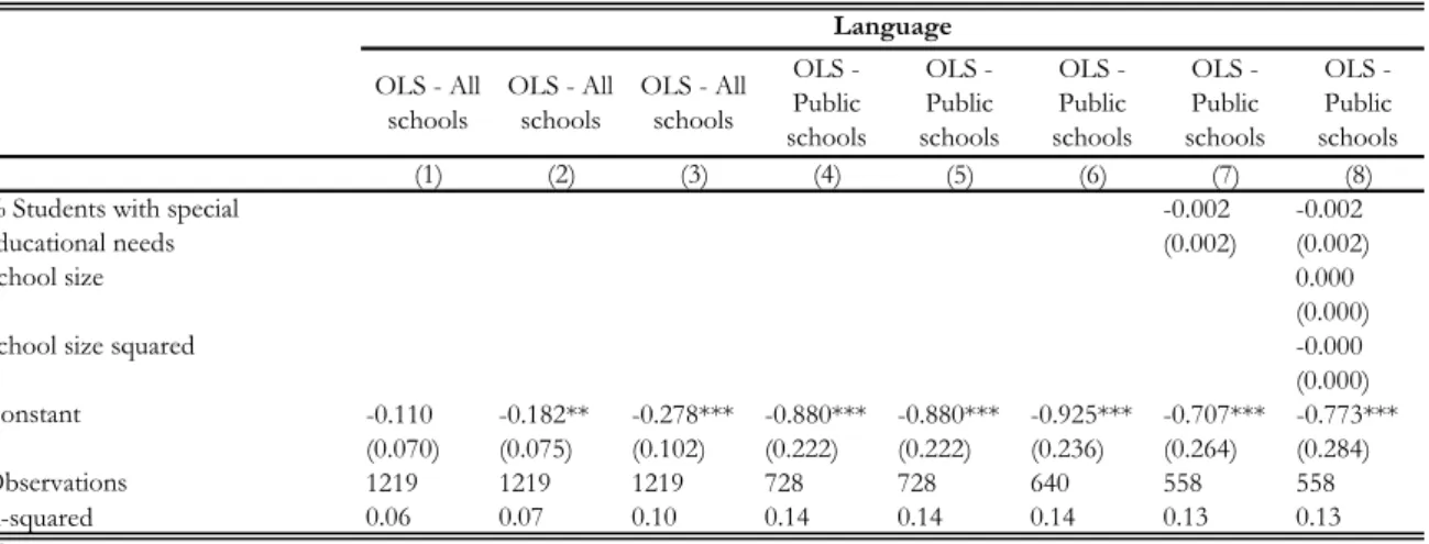
A noteworthy aspect of this project is that we have found some concrete evidence of the importance on parental involvement in the school. The percentage of school activities organized by the Parents’ Association (AMPA)4 has a large and significant effect on the dictation, language and mathematics exams.
The school type (public, private or “concertado”) is important before we control for the family background of class members. More precisely, the impact of private and
“concertado” status on the school fixed effect is highly significant. However, once we control for the socioeconomic composition of the classroom the effect vanishes. This means that these types of schools have been good at separating the children of better educated parents from the rest, and allowing their students to extract the “peer effects” of their classmates.
The remainder of the paper is organized as follows. In section 2 we discuss the relevant literature on the economics of education. Section 3 describes the data and the empirical strategy. Section 4 shows the results. Section 5 concludes.
4Again, for this variable we only have data for public schools.
6
2. THE LITERATURE
The literature on policy interventions in the educational sector is rather vast by now.
In this review, we select a few topics and describe a few papers in each of them. At the end of the section, we offer some preliminary conclusions based on our reading of the evidence.
2.1. School resources
This is probably the kind of intervention that has received the largest amount of attention by economists. There are a couple of reasons for this. One is that it is easy to measure with the current databases. The money spent per student, the number of teachers in a school, are typically available in the data which economists have been able to use. Another important reason is that a first line of defence for administrators whose schools are seen to be floundering is the rallying cry of: “we need more resources”.
Unfortunately, the evidence on this is rather mixed. On a first approximation the case for adding resources or reducing class sizes to improve school performance does not look very strong. Class sizes in many countries have been reduced, dramatically in some cases, over the last few decades, without any noticeable improvement in student performance, measured through standardized testing. For example, Hanushek (1999, 2003) reviews the literature and fails to observe consistent improvements in quality through input-based policies.
This conclusion is controversial. Much of the evidence, as we mentioned, comes from longitudinal databases where it is often difficult to be sure that all relevant variables are included, and firmly establishing causality can be very difficult. For this reason, some researchers have resorted to other forms of analysis that can determine the causal effect of class size in a more robust way.
Probably the least controversial method for analyzing the evidence on class size, or any other policy, is through a field experiment. A group of students is randomly selected to be
“treated” with a smaller class size and their performance is compared to the one of a control group. The most famous experiment in this field is the Tennessee STAR experiment. Finn and Achilles (1990) report gains of about .3 to .6 of a standard deviation in the class mean.
Krueger (1999) reanalyzes the data with more sophisticated econometric techniques and finds somewhat larger gains.5
5 Hanushek (1999b) shows, however, that the experiment was not completely clean. There was attrition from the program (some students “stopped” the treatment) and significant crossover between classes. Furthermore, teachers and students knew they were participating in an experiment, and this could have affected the results.
7
An alternative way of analyzing the problem that has the advantage of being more widely applicable (we will exploit it later in this paper, for example) was introduced by Angrist and Lavy (1999). The authors use the fact that in Israeli schools when the class reaches a ceiling of 40 students, it must be split into two smaller groups. One can use this exogenous split to create instrumental variables, and also to produce a regression discontinuity design, where outcomes are compared at both sides of this boundary. They find an effect that is sizeable. The grades increase by about a third of a standard deviation in the class mean, for reducing the number of students by eight. The effect is clear among fifth graders and (a little bit less) for fourth graders, but virtually non-existent for third graders.
Other researchers, with data from different countries, such as Hoxby (2000) for the U.S. and Leuven, Oosterbeek, Rønning (2008) (and even this paper, for Spain) show that, for their datasets, the effect of class size is statistically indistinguishable from zero. Given the larger initial class size in Israel than in the other places it is not difficult to envisage a situation where class sizes are important at a high level, but become less significant when the base level is reduced.
An important policy in this context, especially in Spain where the government announced plans to do it, is to add computers in classroom. The evidence, however, should make us sceptical about this program. Angrist and Lavy (2002) studied a program, sponsored by the Israeli state lottery, which placed 35,000 computers in schools across Israel between 1994 and 1996. They could find no impact on mathematics or Hebrew standardized exam scores at either the fourth or eighth grade level. Leuven et al. (2007) used data for a program in the Netherlands which gave primary schools with at least 70% pupils from disadvantaged backgrounds extra funding for computers and software. The 70% cut-offs make a regression discontinuity design possible. They find negative point estimates, which are significantly different from 0 for girls’ achievement.
Barrera-Osorio and Linden (2009) report on “Computadores para Educar” an experimental program from Colombia, partnering public and private organizations to introduce computers in the classroom. The program had no impact on students’ math and Spanish test scores. It also failed to increase hours of study, improve the perceptions of school, or relationships with their peers. Interestingly the reason was that although the program was intended to increase the use of computers for teaching, they were mainly used to teach students computers usage skills.
From this short review it is easy to see that the issue remains contentious, and it is not completely settled. Under these circumstances it is difficult to make a recommendation in favour of expensive policies for class reduction size, or to put more computers within the
8
reach of students. In the case of Spain, the main policy tool to deal with students with particularly bad backgrounds or circumstances (“Estudiantes con necesidades educativas especiales” or “Educación compensatoria”) is precisely to teach these students in radically reduced groups (often down to two or three students) for a large fraction of the day. These programs need to be carefully evaluated. A star policy of the government for children in general is to subsidize their usage of computers. As the evidence reported in this section shows, this is probably not the best way to use scarce public funds.
2.2. Teacher’s quality and incentives for all
The situation with teacher’s quality is, in a sense, opposite to the one with resources and school size. Everyone seems to agree that it is very important, on the basis of not much evidence. The problem in this case is that the quality of teachers is very hard to observe. One could, in principle, deduce it from the variation of performance for similarly able kids. But since good students tend to be together (in more technical parlance, there is “assortative matching”), it becomes hard to disentangle the effect of the teachers and other variables.
A very important paper in this context is Rivkin, Hanushek and Kain (2005). Using a very good panel data from the UTD Texas Schools Project they can identify teacher quality based on student performance as well as the impact of some measurable characteristics of teachers and schools. Estimates of the variance in teacher quality based on within-school heterogeneity show that teachers have large effects on reading and mathematics. A one standard deviation increase in teacher quality increases by at least 0.11 standard deviations the total grade in mathematics and 0.095 in reading. A very similar result is obtained by Rockoff (2004) for a different database. Unfortunately, little of the variation in teacher quality is explained by observables such as education or experience, although Rockoff does observe some impact of teachers with more than 10 years experience in the reading grades. These results mean that the practice of rewarding the acquisition of a Master’s degree or the length of tenure in the school system is unlikely to yield any observable gains in the performance of our students.
An immediate implication of the fact that quality is unobservable is that some sort of incentive scheme is necessary to elicit the right kind of teacher quality. This is so both to select and retain the best teachers, as well as to improve their performance. In fact, Lavy (2002) reviews the evidence of a program implemented in Israel in 62 secondary schools in 1995. A sum determined in advance (about $1.4 million) was distributed among the top third performers, in the form of merit raises or a general increase in the quality of professors’
9
facilities. The winners were selected using various achievement criteria, including dropout rates. Although the schools were not chosen randomly, they were chosen according to a criterion (being the only one of its kind in an area) that allows a threshold discontinuity analysis that can control for the non-random selection into the program.
The results show that teachers’ monetary incentives had positive outcomes (especially after the second year) in average test scores, probability of finishing the degree (particularly disadvantaged students) and a reduction in the dropout rate from middle to high school. The results regarding another program, which gives schools resources such as additional teaching time and on-the-job teacher training show that incentives are more cost effective.
Atkinson et al. (2009) use data from a program in the UK. Teachers with a number of years of experience and certain qualifications can apply to pass the Performance Threshold. If they do, they obtain an annual bonus of £2000, payable without revision until the end of their career and included in pension calculations. In addition once over the Threshold, teachers can obtain additional performance based raises. Notice that this program is quite different from the Israeli one. In particular the competitive element is less prominent. Nevertheless, the authors find important effects of the incentive scheme. Teachers that were eligible for the incentive payment increased by almost half a GCSE grade per pupil relative to ineligible teachers, equal to 73% of a standard deviation. They also find significant differences between subjects, with eligible maths teachers showing no effect of the scheme.
Duflo, Dupas and Kremer (2009) use data from a randomized experiment in 140 schools in Western Kenya, half of which received funding to improve the teacher student ratio, by using some extra contract teachers. Students assigned to the contract teachers in the treated schools score 0.18 standard deviations higher than students assigned to the regular teacher in the same schools, possibly due to the different incentives they face. They also score 0.27 standard deviations higher than students in comparison schools. Importantly, in some schools, the school committees were trained to monitor the teachers. In those schools, the students taught by the regular and to the extra teacher do very similarly, and significantly better than students in comparison schools (about 0.21 standard deviations higher in math).
Somebody could argue that an alternative to providing incentives is a good selection of teachers, ex-ante. After all, in Spain there is a very selective exam to obtain the civil service status in the teaching profession. The evidence reported in Angrist and Guryan (2008) induces us to be cautious about this issue. They use the Schools and Staffing Survey to estimate the effect of state teacher testing requirements on teacher wages and teacher quality. The results suggest that state mandated teacher testing is associated with increases in teacher wages, but
10
they are no more likely to be drawn from more selective colleges or to teach material studied in college or graduate school.
Incentives for teachers are not the only way forward. The Mexican Progresa program showed (see e.g. Schultz 2004) that incentives to parents are useful to induce them to let children stay in school. This was an experimental program in which 314 villages were selected randomly (out of a total of 495) to receive the treatment of the program. A grant would be available to poor mothers of a child enrolled in school and confirmed by their teacher to be attending 85% of the school days. These grants were provided for the last 4 years of primary school and the next 3 years of junior high school. The results show that, in primary school, enrolment rates increase by 0.92% for girls and 0.80% for boys, from a initially high level of 94%. In secondary school, the increase is of 9.2% for girls and 6.2% for boys, from their initial levels of 67% and 73%.
Perhaps more important, from the point of view of a more developed economy, is the paper of Angrist and Lavy (2009). They report on an experiment to increase certification rates at the Israeli matriculation certificate, which is a prerequisite for most university level studies.
They offered a prize to all those students in randomly selected schools who passed their exams. This led to an increase in certification rates for girls only (a 10% increase when the mean rate was 29%). The increase in girls’ passing the exam led to higher college attendance.
The main cause for this was extra time dedicated to exam preparation.
Although the evidence on this point is less abundant than the one for school resources, both the existing data, as well as our general economic knowledge about the power of incentives suggests that this is a policy that authorities should implement more generally.
2.3. Parental choice: vouchers, charter schools, and the No Child Left Behind act
A usual recommendation by economists to any resource allocation problem is to introduce competition into the system. Indeed, one of the protagonists of educational reforms in many countries has been the introduction (or more precisely re-introduction) of private providers of education, often with a measure of public funding. The idea is that more parental choice would provide a better match to their preferences and in addition more incentives to all the providers. This is clear for the private ones, since they risk losing the customers if the quality decreases. But the hope was that public schools would also react to the introduction of competition.
One of the most cited instruments to foster competition and parental choice in countries like the US, which already has a large measure of private provision of education, is
11
the disbursement by the government to private schools of an amount per pupil. In principle (but this varies in practice) the schools are free to charge extra fees, so the public expense is a subsidy. This subsidy can be means-tested, i.e., it can depend on parental income, since the idea is that the measure would disproportionately benefit lower-class children whose only option, without the subsidy, is a public school.
There are a few experiments, or quasi experiments with vouchers which help us establish if the theoretically predicted beneficial effects already happen in the field. Angrist et al. (2002) study a natural experiment. The Colombian government had a long run program with vouchers that partly subsidized attendance to private schools, for students that do sufficiently well at school. Since demand for the program was much larger than the supply of grants, the demand was rationed through a lottery. Comparing lottery winners and losers is thus a good identification strategy for the effects of the program. They found that lottery winners are 10% less likely to repeat a grade, and less likely to work (and hence drop out of school. To make sure that this translates in better academic standards, they applied a test to a sample of winners and losers and found that the winners had an average that was 0.2 standard deviations larger than the losers. The cost of the subsidy for authorities were 24$ higher than the provision of a public school place. Hence it seems a relatively cost-effective intervention.
Another important randomized voucher trial took place in New York City. This one was also a subsidy in the form of a 1400$ grant for poor families (those that qualify for a school lunch). In this case, demand also was much larger than supply of the grants and access to them was randomized. The results of this experiment are not very promising. There is certainly no effect for students that are not African American. For African Americans, Howell and Peterson (2002) did find a positive and significant effect. But Krueger and Zhu (2004) find that this effect practically disappears once the students without a baseline grade are included, something that is possible to do without biasing results, and increasing precision, because of the randomized nature of the intervention.
As we mentioned at the beginning of this section, vouchers and other forms of school choice are supposed to affect schools through a competitive effect. Chakrabarti (2008) analyzes the impact of a voucher program on school competition. The Milwaukee voucher program allowed religious private schools to participate for the first time in 1998. After that time there was a large increase in the number of participating schools. Perhaps more importantly, the loss of funding of public schools from the program increased at that time.
Using data from 1987 to 2002, and difference-in-differences estimation for trends, he finds that these changes have led to an improvement of the public schools.
12
One potential problem with vouchers, which cannot show up in experimental evidence, since by its very nature it affects relatively few students, is that large scale voucher programs could end up producing segregation of low income students into purely public schools, potentially harming the same students it is supposed to help most. In this respect there is very little direct evidence, but some important computational work. Epple and Romano (1998) show, in a calibrated general equilibrium model, that vouchers can help low- income high ability students, but through segregation, may harm the remaining poor students.
That model, however, does not allow for residential mobility. Nechyba (2000), on the other hand does allow for mobility in his own model, calibrated to mimic the state of New York. He shows that, indeed, mobility will be large under voucher programs. His results suggest that schemes should be aimed at districts with poor public-school quality, rather than at poor individual households. Urquiola and Verhoogen (2009) obtain similar conclusions for their analysis of the Chilean experience. Their results also show that with school choice there may be different characteristics at both sides of the discontinuity of legally enforced class splits (45 children in Chile), which suggests that regression discontinuity designs may not provide unbiased estimates in a context with significant school choice.
The first bill signed by George W. Bush when he reached the presidency was one of the few bipartisan acts of his presidency, the No Child Left Behind Act (NCLB). In fact, significant parts of it were already designed during the Clinton administration. The two most salient aspects of the bill were its emphasis on school accountability through standardized examinations, research based initiatives and, importantly, parental information and choice as a basis for action. One of the most important provisions of the bill was that parents of public schools that were doing badly (measured by a number of important indicators), would receive information about this failure. They would also be allowed to school their children in other schools from neighbouring school areas where they would, under normal circumstances, not have been allowed to send their children without living there.
Hastings and Weinstein (2008) study the effects of the NCLB act through enhanced parental choice. To do it they use a natural experiment, and a field experiment in North Carolina. From 2002 to 2004, the parental choice was based on a guide with self descriptions from the schools. To find objective statistics required a complicated internet based search.
From 2004 the school district sent a spreadsheet with detailed objective statistics. That is the natural experiment, which is used to observe the effect of information on school choice and also of school changes for those who shift schools. In addition, the authors did a field experiment with random choice of school and information recipients. In the field experiment the information was easier to read and better targeted to the parents.
13
In both experiments, it was found that providing clear, direct information resulted in an increased choice of higher ranked schools by parents. About 5 to 7 percent more parents (from a base of about 16 percent) chose to change schools. The parents who chose to change schools sent their children to schools that, on average, were about half a standard deviation better than the previous ones. Those kids who do move to a new one made gains that are marginally significant. The point estimates of these gains suggest a gain of about 0.3 standard deviations, when changing to a school with a one standard deviation higher average.
Another interesting experiment having to do with choice is the Moving to Opportunity program, implemented by the Housing and Urban Development department in five American cities in the 90s. This program subsidized families living in high poverty areas to move to areas with lower poverty and crime rates. Kling, Liebman and Katz (2007) find that this program led to positive effects for female youth on education, (as well as risky behavior and physical health). However, the effects for male youth were negative.
For school resources we found that they probably do not matter much, and for teacher’s quality we concluded that it definitely matters, and we have good ideas for how to improve it. In the case of school choice, we find that it may be a positive force, but it carries a risk of social polarization and, in any case, a lot depends on details of implementation. For Spain, there is already a fair amount of school choice, but it is clear that it does not reach sufficiently those that need it most. The No Child Left Behind act points to a good way forward.
2.4. Other policies: early intervention, streaming/tracking
An important issue when resources are limited is where, and who, to target. In this respect there is a notable set of long-running policy experiments reported in Heckman (2008).
These experiments show, in the words of the author that “high quality early childhood interventions foster abilities and that inequality can be attacked at its source. Early interventions also boost the productivity of the economy.”
The experiments mentioned in the previous paragraph are the Perry Preschool Program and the Abecedarian Program. They are useful because they are conducted in a careful randomized fashion, but also because they collect long-term data (even after the treatment ended) of the effects on treated and non-treated individuals on schooling achievement, job performance, and social behaviours, long after the interventions ended. The Perry Program consisted in a 2.5 hour daily classroom session as well as a weekly 90 minute visit home by a teacher. The participants were 58 poor black children in Michigan between
14
1962 and 1967, for 30 weeks a year. The treated and control groups were followed until age 40. The Abecedarian Program studied 111 children, whose families scored high on a social risk index. The average entry age was 4.4 months. This program was more intensive. It lasted the whole year and the attention was provided for the whole day. The treated children were followed until age 21.
Data from the programs suggest that initial IQ increases disappear over time, but school attainment is clearly higher. For example, in the Perry program percentage of students in special education halves (from 34% to 15%) in the treatment group compared to the control, the percentage above the 10 percentile more than triples (from 15% to 49%) and the percentage who graduate on time from high school goes from 45% to 66%. This translates into a much higher proportion who earns more than 2000$ a month (from 7% to 28%), owns a home (13% to 36%) or is never on welfare (from 14% to 29%). The reduction of crime rates among these children is also dramatic, as the proportion of arrests roughly halves. Heckman et al. (2008) calculate a rate of return for this program of about 10%.
The experimental evidence from early intervention and the detailed studies of Heckman and his co-authors on the formation of non-cognitive abilities and labor market outcomes (see, for instance Heckman 2007, or Cunha and Heckman 2009) suggest that the Spanish preschool programs are probably worth pursuing. But given their cost, we would suggest to focus even more strongly on the children who are more at risk and to enrich them with interventions out of the classroom.
Another policy intervention that is sometimes discussed in the public policy arena consists of grouping students by ability levels. Early evidence from longitudinal databases seemed to indicate that this policy measure was good for high-ability students, but it hurt lower ability students who did not have anymore the advantage of profiting from better performing peers. A re-analysis of earlier studies by Betts and Shkolnik (2000), however, suggests that this early impression was probably wrong and a strong conclusion was not warranted. They mention a series of problems with the comparisons. For example, ability is measured imperfectly and hence the grouping is not quite homogeneous. Some schools do not use ability grouping officially, but may do it informally. In some databases, teachers are asked to identify a class as “above average”, “average”, “below average”, or “heterogeneous”. But it is not clear what the variation in ability is in “heterogeneous” groups. Sometimes surveys do not distinguish between ability grouping, or channelling students into different curricular tracks. Tracking schools could allocate more resources to lower ability groups, thus confounding the effects of resources and tracking. Finally, it is possible that students are tracked in groups even within a classroom.
15
Given all the above problems with the databases, the recent study of Duflo, Dupas and Kremer (2008) is very meaningful. They compare 61 Kenyan schools in which students were randomly assigned to a first grade class with 60 in which students were assigned based on initial achievement. Students in tracking schools scored 0.14 standard deviations higher (after 18 months) than those children in non-tracking schools, and the effect remained after the program ended. Interestingly students at all levels of the distribution benefited from tracking.
Thus, since the same study also shows that direct effect from higher ability peers is positive, tracking must affect lower- performing students by allowing teachers to modulate the level of the class better.
In this case the evidence is far from conclusive, but it is sufficiently suggestive to warrant a recommendation for some trial (experimental) programs for tracking.
3. DESCRIPTION OF THE DATA
The data for our empirical analysis comes from a standardized exam that is administered each year to the 6th grade students6 (around 12-13 years old7) of all primary schools (about 1200) in the region of Madrid. The exam is called “prueba C.D.I. - prueba de Conocimientos y Destrezas Indispensables”. This exam was introduced by the Education Council of the region of Madrid in the academic year 2004/2005, and it is obligatory for all primary schools (public, private or charter). The exam does not have academic consequences for the children. It is intended to give additional information to the children and their families as well as to the educational authorities.
We have the scores of this exam for four cohorts of students in the academic years 2005/2006, 2006/2007, 2007/2008, 2008/2009.8
The exam consists of two parts of 45 minutes each: the first part includes tests of dictation, reading, language and general knowledge and the second part is composed of mathematics exercises. Our measures of student achievement are the standardized scores to the yearly mean in each of these five subjects.
6The Spanish educational system is composed of 6 years of primary school, 4 years of compulsory secondary education (E.S.O.) and 2 years of non-compulsory education, which is divided into vocational training (ciclos formativos) and preparation for college (bachillerato).
7In primary school, students can repeat a grade in case their performance is deemed insufficient. On average, in the whole of Spain, the percentage of repeaters is 6.2%. Madrid is close to the national average with 6.5%. For more statistics and details on the Spanish educational system, see e.g.
http://www.institutodeevaluacion.mec.es/contenidos/indicadores/ind2009.pdf.
8Results for the year 2004/2005 are available as well. However, we do not use them in this paper since for this year there was no information on the individual characteristics of the students.
16
Additionally, in 2009 a short questionnaire (see Appendix) was filled out by each student. In the questionnaire the students were asked a few questions about themselves, their parents and the environment in which they are living. The answers to this questionnaire provide rich information on the individual characteristics of the students that is not available for the previous cohorts; therefore we focus our empirical analysis on this cohort. Results of the estimations using the data set composed of the three cohorts of students from the years 2006-2008 are conducted as a robustness check and are provided in the Appendix of the paper.
Since the performance of the children is a combination of individual and family characteristics and school resources, we distinguish two categories of control variables:
variables at individual level (student characteristics and family background) and variables at school level. The availability of the data at these two levels of aggregation will justify our econometric methodology (see next section).
The individual level variables that are common for all four cohorts are: gender, nationality (Spanish or immigrant), whether the student has special educational needs and whether the student has any disability.
For the 2009 cohort the set of control variables at individual level is significantly larger. The questionnaire provides the following variables: the age of the student, the country of birth (Spain, China, Latin America, Morocco, Romania and other), the level of education of the parents, the occupation of the parents, the composition of the household in which the student lives and the age at which the student started to go to the school.
Regarding the education of the parents, students were asked to provide this information for both the mother and the father. However, to facilitate the interpretation we choose the highest level of education between the mother and the father. We distinguish the following categories: university education, higher secondary education, vocational training, lower secondary education and no compulsory education.
In the case of the occupation of the parents, we apply the same strategy as for the education: we choose the highest level of occupation between the mother and the father.
Accordingly, we differentiate between the following categories: professional occupations (for example teacher, researcher, doctor, engineer, lawyer, psychologist, artist, etc.), business and administrative occupations (for example CEO, civil servants, etc.) and low-skilled occupations (for example shop-assistant, fireman, construction worker, cleaning staff, etc.).
The composition of the household in which the student lives is constructed according to the answers to the question: “With whom do you usually live?”. We differentiate the following 7 categories: lives only with the mother, lives with the mother and one
17
brother/sister, lives with the mother and more than one brother/sister, lives with the mother and the father, lives with the mother and the father and one brother/sister, lives with the mother and the father and more than one brother/sister and other situations.
The school level variables that are available for all schools (public, private and charter) are the following: class size, enrollment in the 6th grade and the geographical location of the school in the region of Madrid (East, West, North, South or Capital). Additionally, from the data at student level we compute the share (percentage) of immigrants in the class and the shares (percentages) of students with parents with a certain level of education in the class (university, higher secondary, vocational training, lower secondary and didn’t finish compulsory studies).
The school level variables that are available only for public schools are the following:
teacher/student ratio, average age of the teachers, share of extra-curricular activities organized by Parents’ Associations, share of students that are eligible for a free meal, school size, share of students with special educational needs.
Class size is calculated as the total number of students enrolled in the 6th grade divided by the total number of 6th grade classes. Enrollment in the 6th grade is the total number of students registered in the 6th grade. Teacher/student ratio is the ratio of the number of professors teaching in the 6th grade classes and the number of students enrolled in the 6th grade. Average age of the teachers is the average age of the professors teaching in the 6th grade. Share of extracurricular activities organized by Parents’ Associations is the percentage of these activities in the total number of extracurricular activities in a school. Share of students that qualify for a free meal and share of students with special educational needs is the percentage of students in the 6th grade with one of these characteristics.
The data set for the 2009 cohort is formed of 56,929 students in 1,227 public, private and charter schools. Out of this number, 735 are public schools. However, due to data availability, we use in our estimations a sample of about 44,500 students in 1,222 schools for the individual level regressions and a sample of 558 public schools for the school level estimations.9
The descriptive statistics of the student and school data are presented in Tables 1 and 2.
9 The data set for the 2006-2008 cohorts is composed of a total of 155 226 students in 1,237 public, private and charter schools (around 50,000 students in each year). Out of these schools, 735 are public schools.
18
Variable Mean Std. Dev. Min Max
Subjects
Dictation 0.12 0.94 -1.60 1.27
Mathematics 0.13 0.94 -1.77 1.94
Language 0.15 0.90 -2.04 1.71
Reading 0.14 0.91 -1.97 1.39
General knowledge 0.12 0.94 -1.66 1.88
Individual characteristics
Female 0.49 0.50 0 1
Student with special educational needs 0.06 0.23 0 1
Student with disability 0.02 0.14 0 1
Student's age 12.13 0.40 10 17
Student Spain 0.82 0.38 0 1
Student Romania 0.02 0.15 0 1
Student Morroco 0.01 0.09 0 1
Student Latin America 0.10 0.30 0 1
Student China 0.00 0.07 0 1
Student other 0.04 0.20 0 1
Parent education - Univ. 0.48 0.50 0 1
Parent education - Higher secondary 0.17 0.38 0 1
Parent education - Vocational training 0.12 0.32 0 1
Parent education - Lower secondary 0.17 0.38 0 1
Parent education - didn't finish compulsory
studies 0.06 0.23 0 1
Parent occupation - Business, minister, city hall,
CCAA 0.22 0.42 0 1
Parent occupation- Professional 0.34 0.47 0 1
Parent occupation - Blue Collar 0.44 0.50 0 1
Lives only with the mother 0.07 0.25 0 1
Lives with the mother and one brother/sister 0.04 0.20 0 1 Lives with the mother and more than one
brother/sister 0.02 0.13 0 1
Lives with the mother and the father 0.16 0.37 0 1
Lives with the mother and the father and one
brother/sister 0.43 0.50 0 1
Lives with the mother and the father and more
than one brother/sister 0.17 0.37 0 1
Other situations 0.11 0.32 0 1
Start school before 3 0.53 0.50 0 1
Kindergarden between 3 and 5 0.44 0.50 0 1
Start school at 6 0.02 0.15 0 1
Start school at 7 or more 0.01 0.11 0 1
Observations 44542
Table 1
Descriptive statistics of individual level variables 2008/2009 cohort
19
Variable Mean Std. Dev. Min Max
Subjects
Fixed effects - Dictation 0.05 0.43 -1.50 1.43
Fixed effects - Mathematics -0.03 0.36 -1.60 1.62
Fixed effects - Language -0.07 0.38 -1.56 0.99
Fixed effects - Reading -0.16 0.35 -1.43 1.11
Fixed effects - General knowledge -0.26 0.45 -1.41 1.72
School characteristics All schools
Class size 23.40 3.89 2.00 34.00
Enrollment 6th grade 49.49 23.37 2 177
% Immigrant students in 6th grade (0-10% 0.38 0.48 0 1
% Immigrant students in 6th grade (11-20%) 0.28 0.45 0 1
% Immigrant students in 6th grade (21-30%) 0.17 0.37 0 1
% Immigrant students in 6th grade (31-40%) 0.09 0.28 0 1
% Immigrant students in 6th grade (>40%) 0.09 0.28 0 1
% Parent's education - Univ. 34.25 20.02 0.00 100.00
% Parents' education - Higher secondary 15.70 8.19 0.00 52.38
% Parents' education - Vocational training 10.02 6.17 0.00 62.50
% Parents' education -Lower secondary 16.16 10.78 0.00 75.00
% Parents' education - didn't finish compulsory
studies 5.52 5.87 0.00 72.00
School Capital 0.40 0.49 0 1
School East 0.14 0.35 0 1
School North 0.08 0.26 0 1
School West 0.10 0.30 0 1
School South 0.29 0.45 0 1
Public schools
Teacher/student ratio 0.26 0.15 0.08 1.67
Av. age teacher 43.09 4.46 29.11 57.78
No. AMPA activ./total no. of activ. 0.06 0.15 0.00 1.00
% Students free meal 13.23 9.28 0.15 48.57
School size 382.71 149.34 18.00 1088.00
% Students with special educational needs 11.40 10.63 0.00 55.56 Table 2
Descriptive statistics of school level variables 2008/2009 cohort
20
4. ECONOMETRIC METHODOLOGY AND RESULTS
Since we handle data at two levels of aggregation (data at individual level and data at school level), we use a two-stage estimation procedure in order to model the relationship between student and school characteristics and academic outcomes, a strategy that has been often followed by previous research (Loeb and Bound, 1996, Hanushek et al., 1996).10
The first stage is an OLS regression in which the standardized grades of the students in all the schools are regressed against individual characteristics and school dummies (school fixed effects). The coefficients on the school dummies can be interpreted as the value added of the school, once differences in student characteristics are controlled for. The equation that we estimate is the following:
∑
++ +
=
j
ij ij j ij
ij X D u
Y α β δ
where i is the student and j is the school. Xij are individual characteristics of the student described in the previous section (like gender, nationality, etc.). Dij is a school dummy variable that equals 1 if student i attends school j in the academic year 2008/2009.11
The second stage is an OLS regression in which the coefficients of the school dummies (δj) are regressed against the school level variables:
j j
j =γ +θZ +v
δ
where Zj are school level variables. Because of large differences among schools sizes, we believe that there could be potential efficiency gains from weighting the data by an estimate of the covariance matrix. Therefore, the second stage estimations are weighted by the inverse of the estimated variance of the school fixed effects from the first stage. In the Appendix, Tables A1-A3, we report the results from the unweighted regressions as well.
4.1. First stage results
Table 3 reports the results for the first stage regressions, for the 2009 cohort. The dependent variables are the individual standardized grades in each of the five tests. All
10According to Hanushek et al. (1996), aggregation of the data inflates the coefficients on school resources. Moreover, their empirical analysis proves that problems associated with omitted variables bias tend to aggravate along with the level of aggregation. This causes studies that use more aggregated data to overestimate the effect of school resources on academic performance. In particular, they show that this is the case for studies that use data for US schools aggregated at state level.
The less aggregated the data is, the more likely it is that they will produce reliable estimates of the school resources on academic performance. This argument comes in our favor since our most aggregated data is at school level.
11 For the 2006-2008 panel, one should add a cohort (time) index for the variables from this specification.
21
regressions include school dummy variablesDij. Their coefficients δj are the average school effects once we account for individual characteristics.
Results are in general robust among the five tests, however some differences arise.
In particular, we find that girls do better in dictation and language than boys: on average girls get about 0.2 standard deviations more in dictation and 0.09 standard deviations more in language than boys. On the other hand, in mathematics, boys get on average 0.15 standard deviations more than girls, and in general knowledge they get 0.18 standard deviations more than girls.12 Children with special educational needs and children with any disability perform, on average, quite poorly: they get between a half and one standard deviation less in all the subjects.
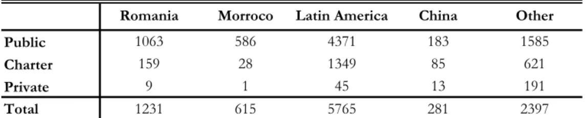
For this cohort, we could control for the country of birth of the immigrant children, therefore we could indentify differences by the country of birth of the children. We distinguish the following groups: Latin America (Ecuador, Colombia, Peru, Bolivia, and Dominican Republic), Romania, Morocco, China and other countries. The groups that we choose correspond to the largest groups of immigrants in Spain, and, also, from the region of Madrid. According to the last census in Spain (January 2009), out of the 5.6 million foreigners in Spain around 1 million live in the region of Madrid. From them, around 33% are from Latin America countries, 19% are from Romania, 8% are from Morocco and around 4% are from China (these groups sum to approximately 63% of the total of immigrants in the region of Madrid).13
We find that once we control for individual characteristics like parental education and occupation, on average immigrants do worse than nationals, however this is not always the case. Children from China do very well in mathematics (approximately one half of a standard deviation better than Spanish children), while children from Romania perform relatively better in dictation, mathematics and language (around 0.08 standard deviations better than Spanish children).
On the other hand, we find no significant difference between Moroccan students and Spanish students in mathematics and general knowledge, while in dictation, reading and language Moroccan perform worse. Children from Latin America are the group with the worst outcomes. They do significantly worse than Spaniards in all the parts of the exam. More concretely, the difference between Latin American and Spanish students equals around 0.25-
12This result is not so surprising if we look at the international results of TIMMS 2007 (Trends in International Mathematics and Science Study) in mathematics. In the 4th grade, boys had higher average achievement than girls in 12 countries, including United States, Sweden, Norway, Scotland, Netherlands, Germany, Austria, and Italy.
13These numbers take into account the nationality of the person.
22
0.27 standard deviations less in dictation and language and around 0.2 standard deviations less in mathematics and general knowledge.
The age of the student appears to matter as well: the younger the child, the better he performs in all the tests. The effect of the age is negative and statistically significant even after controlling for nationality (there might be immigrants that don’t have the necessary knowledge to be in a grade according to their age) and for children with special educational needs or children with some disability.
Both parental education and occupation are extremely important, confirming results from previous studies. If we compare the magnitude of the coefficients, the level of education appears to matter more than the profession of the parents. The effect of education is the highest in the case of children whose parents have a university degree, in all the subjects: in mathematics, the difference between a child with a parent that has a university degree and a child with a parent that has no studies is about 0.2 standard deviations. This difference decreases in magnitude as the level of education of the parents decreases, but it remains statistically significant.
Students whose parents have professional occupations (for example, teacher, researcher, doctor, engineer, lawyer, psychologist, artist, etc.) do significantly better than the rest. The coefficient for this dummy is approximately twice the coefficient for the dummy for parents with white collar occupations (like CEOs or civil servants). This might indicate that parents with professional occupations are likely to place a greater value on education than the rest.
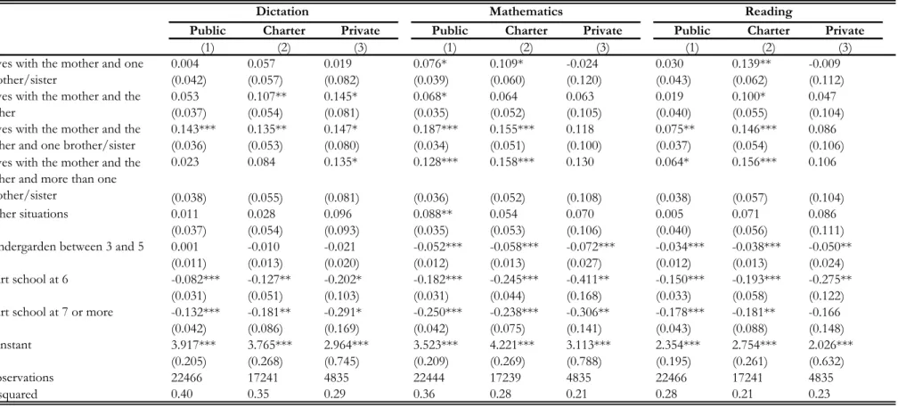
The estimations reveal also that living with both the mother and the father is beneficial for the performance of the children in schools. Moreover, it appears that having brothers or sisters improves student outcomes.
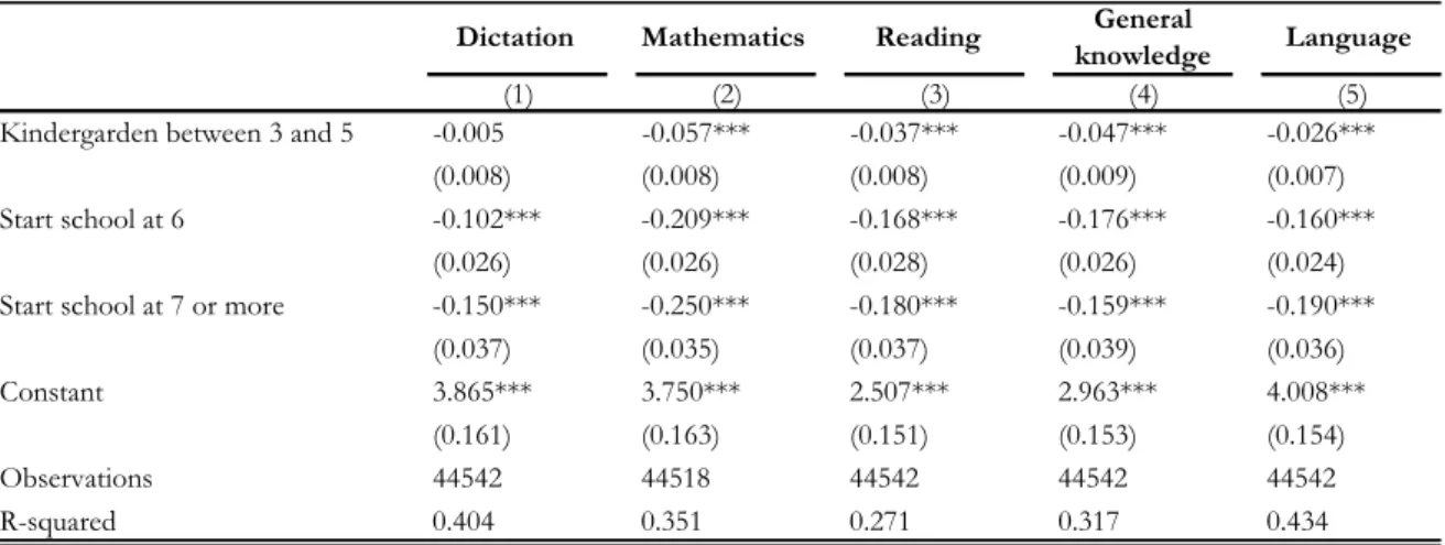
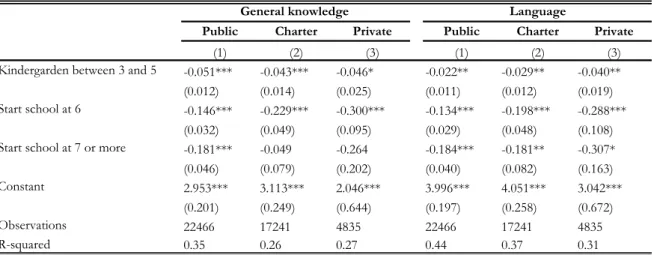
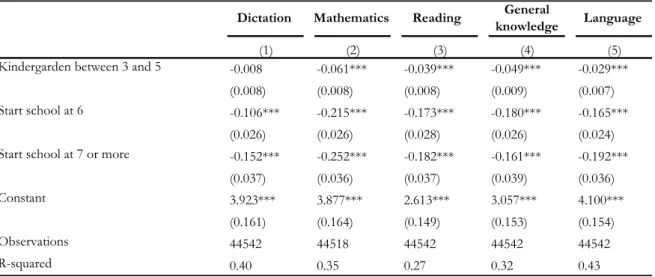
There is also empirical evidence for the fact that starting to go to school at an early age is beneficial for the school performance of the children. A child that has started to go to school at less than 3 years of age gets around 0.2 standard deviations more in the CDI exam than a child that has started to go to school at 7 years or more.
To summarize the results of the first stage, we can draw the following conclusions.
Girls do relatively better in dictation and language and relatively worse in mathematics and general knowledge, when compared to boys. The performance of immigrant children is, in general, poorer than of the Spanish students, controlling for the family background of the children. However, there are exceptions: Chinese students perform very well in mathematics;
they get on average about one half of a standard deviation more than Spanish students and Romanian students perform, on average, better than Spanish students in all the subjects
23
(except in general knowledge). We also find that the younger the student, the better she will perform in school and that starting the school at an early age is also very beneficial for the student’s performance. The education and the profession of the parents appear among the most important determinants of the academic performance of children. If we compare the magnitude of the coefficients, the effect of the education of the parents is stronger than the effect of the profession.
24
Dictation Mathematics Reading General
knowledge Language
(1) (2) (3) (4) (5)
Female 0.213*** -0.148*** -0.003 -0.181*** 0.090***
(0.008) (0.008) (0.008) (0.009) (0.007)
-0.761*** -0.736*** -0.561*** -0.551*** -0.799***
(0.021) (0.020) (0.021) (0.020) (0.019)
Student with disability -0.887*** -1.011*** -0.877*** -0.758*** -1.024***
(0.031) (0.030) (0.033) (0.032) (0.031)
Student's age -0.330*** -0.314*** -0.211*** -0.245*** -0.339***
(0.013) (0.013) (0.012) (0.012) (0.012)
Student Romania 0.079** 0.081*** 0.053* 0.045 0.078***
(0.032) (0.030) (0.031) (0.031) (0.030)
Student Morroco -0.194*** 0.014 -0.153*** -0.030 -0.177***
(0.042) (0.039) (0.045) (0.046) (0.039)
Student Latin America -0.273*** -0.199*** -0.064*** -0.206*** -0.251***
(0.016) (0.015) (0.015) (0.016) (0.014)
Student China -0.228*** 0.500*** -0.121 -0.198*** -0.235***
(0.066) (0.077) (0.075) (0.068) (0.068)
Student other -0.077*** -0.106*** -0.013 -0.097*** -0.080***
(0.020) (0.021) (0.020) (0.020) (0.018)
Parent education - Univ. 0.160*** 0.261*** 0.194*** 0.214*** 0.215***
(0.021) (0.019) (0.022) (0.019) (0.020)
0.099*** 0.148*** 0.131*** 0.153*** 0.142***
(0.021) (0.018) (0.022) (0.019) (0.019)
0.083*** 0.135*** 0.142*** 0.159*** 0.136***
(0.023) (0.020) (0.023) (0.021) (0.021)
0.051** 0.080*** 0.078*** 0.072*** 0.074***
(0.021) (0.018) (0.022) (0.019) (0.019)
0.075*** 0.090*** 0.065*** 0.093*** 0.092***
(0.012) (0.012) (0.011) (0.012) (0.010)
Parent occupation- Professional 0.132*** 0.163*** 0.122*** 0.157*** 0.161***
(0.011) (0.011) (0.011) (0.012) (0.010)
Lives only with the mother -0.042 -0.058* -0.032 -0.054 -0.050*
(0.031) (0.030) (0.032) (0.033) (0.028)
0.025 0.079** 0.062* 0.030 0.042
(0.031) (0.032) (0.034) (0.035) (0.029)
0.081*** 0.068** 0.047 0.091*** 0.090***
(0.029) (0.028) (0.030) (0.032) (0.026)
0.137*** 0.168*** 0.097*** 0.119*** 0.148***
(0.028) (0.027) (0.029) (0.031) (0.025)
0.058** 0.143*** 0.098*** 0.078** 0.086***
(0.029) (0.028) (0.030) (0.031) (0.027)
Other situations 0.025 0.076*** 0.032 0.039 0.035
(0.029) (0.029) (0.031) (0.032) (0.026)
Table 3
Pooled OLS with school fixed effects (1st stage) for 2008/2009
Student with special educational needs
Parent education - Higher secondary Parent education - Vocational training
Parent education - Lower secondary Parent occupation - Business, minister, city hall, CCAA
Lives with the mother and one brother/sister
Lives with the mother and the father Lives with the mother and the father and one brother/sister
Lives with the mother and the father and more than one brother/sister