TESTING OPVAR ACCURACY: AN EMPIRICAL BACK-TESTING ON THE LOSS DISTRIBUTION
APPROACH
JOSÉ MANUEL FERIA-DOMÍNGUEZ ENRIQUE J. JIMÉNEZ-RODRÍGUEZ
Mª PAZ RIVERA-PÉREZ
FUNDACIÓN DE LAS CAJAS DE AHORROS DOCUMENTO DE TRABAJO
Nº 693/2012
De conformidad con la base quinta de la convocatoria del Programa de Estímulo a la Investigación, este trabajo ha sido sometido a eva- luación externa anónima de especialistas cualificados a fin de con- trastar su nivel técnico.
ISSN: 1988-8767
La serie DOCUMENTOS DE TRABAJO incluye avances y resultados de investigaciones dentro de los pro- gramas de la Fundación de las Cajas de Ahorros.
Las opiniones son responsabilidad de los autores.
TESTING OPVAR ACCURACY: AN EMPIRICAL BACK-TESTING ON THE LOSS DISTRIBUTION APPROACH
José Manuel Feria-Domínguez*
Enrique J. Jiménez-Rodríguez Mª Paz Rivera-Pérez ABSTRACT
The application of the Value at Risk (VaR) concept to the Loss Distribution Approach (LDA) is encouraged by the Basel Committee for measuring the operational risk. Moreover, complementary analysis such as the back testing exercise plays an important role in assessing the excedancees beyond Operational Value at Risk (OpVaR) forecasts and providing with valuable feedback on the soundness of such advanced measurement approach (AMA).
In this paper, we conduct an empirical back-testing analysis on the LDA by using an Internal Operational Losses Database (IOLD) provided by a medium sized Spanish Savings Bank. We apply different techniques for carrying out the back-testing exercise: the Basic Analysis and Extremal Index, and more complex statistical methods such as Kupiec and Christoffersen’s Tests. Our empirical results bring into light that the application of the LDA model for the Savings bank analyzed would be rejected according to the regulatory framework.
Keywords: Operational Value at Risk; Back-testing; Basel III; Loss Distribution Approach;
Regulatory Capital.
JEL classification: G21; G28; C52.
Corresponding author:
José Manuel Feria-Domínguez, PhD. Department of Financial Economics and Accounting, Pablo de Olavide University, Seville, Spain, 41013. Phone +34 954 977 814. Email:
Acknowledgements: The authors would like to thank the discussants at the 4th International Workshop on Risk Management and Insurance (RISK 2011) and the 19th Multinational Finance Conference (2012) for their valuable comments and suggestions to improve the quality of this paper.
1. INTRODUCTION
Since ages, financial institutions have been exposed to financial risks such as credit and market risk, but also to operational risk (henceforth, OR) whose measurement and control have recently gained significant attention for regulators, supervisors, managers, and investors.
Surprisingly, there has been a lack of consensus on a standard definition for operational risk.
Moreover, it has been considered the firm’s residual risk after other sources of risk, such as market risk and credit risk (Allen & Bali, 2007b). In practice, operational risk differs from other types of risk in being substantially unlimited and potentially large enough to threaten the existence of affected institutions (Cummins, Lewis, & Wei, 2006).
In 2006, with the publication of the document International Convergence of Capital Measurement and Capital Standards document (Basel II), the Basel Committee on Banking Supervision (henceforth the Committee) introduced an explicit definition of such financial risk, somewhat more narrowly than the residual risk concept, as follows: ‘‘the risk of loss resulting from inadequate or failed internal processes, people, and systems or from external events’’. In addition, the main novelty of this international regulatory framework was the introduction of capital charges for covering operational risk, modifying, in consequence, the traditional solvency coefficient. The current financial crisis has forced the Basel Committee to revise those international standards for banking regulation given rise to Basel III. These consultative documents formed the basis of the Committee's response to the financial crisis and are part of the global initiatives to strengthen the financial regulatory system that have been endorsed by the G20 Leaders. More specifically, it implies a set of reform measures in order to strengthen the regulation, supervision and risk management of the banking sector with the aim of:
improving the banking sector's ability to absorb shocks arising from financial and economic stress, whatever the source, improving risk management and governance and strengthening banks' transparency and disclosures.
In practice, the heterogeneity of factors surrounding operational risk increases the complexity when measuring, controlling and managing such a risk within a financial institution.
Being aware of that, the Committee proposes three main methodologies (Basic Indicator, Standardized Approach and Advanced Measurement Approaches) to calculate capital requirements for covering operational risk. In this paper, we will focus on the most sophisticated one, that is, the Loss Distributions Approach (henceforth, LDA), which is an actuarial model to which the Value at Risk (VaR) concept is applied. Inherited from market risk, this is a statistical estimate that indicates the maximum operational loss, expressed in economic terms, in which a bank can incur within a certain period of time (one year) for a given confidence level (99.9%).
Moreover, apart from estimating the corresponding Operational Value at Risk (OpVaR), “banks should also regularly review actual performance after the fact relative to risk estimates (i.e.
back-testing) to assist in gauging the accuracy and effectiveness of the risk management process and making necessary adjustments” (Basel Committee, 2010). In other words, it is
essential to conduct complementary analysis on the internal risk model to demonstrate its soundness.
The main objective of this paper is to carry out an empirical back testing analysis on the LDA model by using an Internal Operational Losses Database (IOLD) provided by a medium sized Spanish Saving Bank prior to be merged in 2007. Our main contribution to the previous research is the transposition of market risk back testing exercise to the operational risk context.
In particular, we test the accuracy of the LDA model, calculating not only the operational capital charges (so called Capital at Risk, CaR) but also assessing the reliability of such statistical estimates. Since there is no specific guidelines for conducting the OR back-testing as in the case of market risk, the topic is challenging because:
The estimation process differ significantly between market VaR and OpVaR as the corresponding models follow different stochastic processes, the former continuous and the latter discrete.
Market VaR estimates are validated against daily profit and loss of a certain portfolio, whereas the OpVaR needs to be tested against the losses themselves.
The market position can be validate every day by marking-to-market while operational losses are detected and recorded with a time lag, that is, one or more days later. In that senses OpVaR is more subject to jumps than the market VaR.
More specifically, we apply different techniques for carrying out the back-testing exercise: the basic analysis, based on the Binary Indicator (BI) and Extremal Index (EI), to more complex statistical methods such as Kupiec and Christoffersen’s Tests.
The paper is organized as follows: In section 2, we describe the sample and data, in section 3, the LDA methodological approach is applied to the data set, in section 4 the back- testing based on the basic analysis is conducted and the statistical analysis is presented in section 5. Finally, our main conclusions are highlighted in section 6.
2. SAMPLE AND DATA
Our clinical study relies on the Internal Operational Data Base (IOLD) provided by a medium sized Spanish Savings Bank which operates within the retail banking sector prior to be merged in 2007. In particular, we have selected one year horizon as a mobile temporal window to estimate 31 daily Operational Value at Risk (OpVaR) as the platform for calibrating the soundness of such statistical estimates.
Firstly, we start considering 6,479 operational risk events recorded between 30/11/05 till 30/11/06 to estimate the first daily OpVaR (30/11/06), that is, the maximum operational loss we expect to occur one day hence with 99.9% of statistical confidence. By rolling over the temporal window (one day ahead in, last day out) we design thirty observation periods ending at 31/12/2006 to which we apply the Loss Distribution Approach (LDA). This is the starting point to carry out the back testing process.
When handling with the data set we should point out that:
In order to avoid the inflation risk, we have used the CPI (Consumer Prices Index) to adjust the amount of the losses, taking the year 2006 as the benchmark. Thus, we have converted the nominal losses in the corresponding equivalent monetary units.
The data have been rescaled for ensuring the identity of the financial institution.
Once we have defined the temporal window, it is essential to perform an EDA (Exploratory Data Analysis) of the data for analyzing the nature of the sample itself (Hoaglin, Mosteller, &
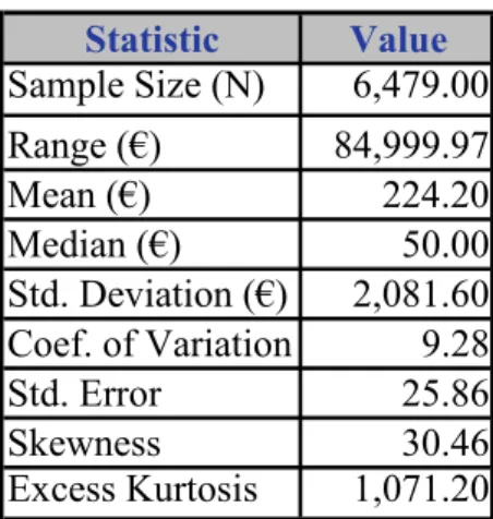
Tukey, 1983; Tukey, 1977).The descriptive statistics are given in the Table 1:
Table 1: Descriptive statistics
Statistic Value Sample Size (N) 6,479.00 Range (€) 84,999.97
Mean (€) 224.20
Median (€) 50.00
Std. Deviation (€) 2,081.60 Coef. of Variation 9.28
Std. Error 25.86
Skewness 30.46
Excess Kurtosis 1,071.20
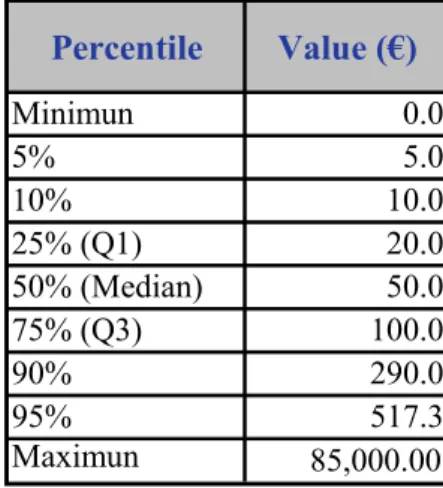
From observing table above, it should be noted that the mean is much higher than the median, what indicates a clear positive asymmetry of the distribution. The descriptive analysis describes a typical operational risk distribution which is characterized by a grouping, in the central body, of low severity values, and a wide tail marked by the occurrence of infrequent but extremely onerous losses, as the Table 2 below illustrates:
Table 2: Percentiles of the Operational Loss Distribution
Percentile Value (€)
Minimun 0.0
5% 5.0
10% 10.0
25% (Q1) 20.0
50% (Median) 50.0
75% (Q3) 100.0
90% 290.0
95% 517.3
Maximun 85,000.00
3. THE LOSS DISTRIBUTION APPROACH (LDA)
Although the application of any Advanced Measurement Approach (AMA) is in principle opened to any proprietary model, the most popular methodology is by far the loss distribution approach (LDA), a parametric technique included under the previous scheme as an actuarial model, which we can be resumed in the following four steps:
Estimating a frequency distribution the number of loss events during a certain time period.
Estimating a severity distribution for the impact of the event in terms of financial loss.
Checking the goodness of fit of previous distributions.
Convoluting of frequency and severity distributions by using Monte Carlo Simulation technique, obtaining the Aggregated Loss Distribution. From the resulting Aggregated Loss Distribution we can determine a minimum capital requirement through a certain percentile, that is, OpVaR.
Modelling the Frequency Distribution
Frequency of operational losses represents a discrete phenomenon. We assume that the number of events between times t and t
, where in a certain time horizon (daily horizon), corresponding to a business line (i) and an event type (j) is a random variable, Nij, with a probability function pij.The loss frequency distribution Pij corresponds to:
nk ij
ij
n p k
P
0
) ( )
(
i17, j18 (1) For the frequency distribution of losses, a Poisson process was initially proposed by Basel (2001a). Later, non-homogeneous versions of the Poisson process for operational risk were proposed and tested with real data (Chernobai, Menn, Rachev, & Trûck, 2006). Negative Binomial distribution was used (Moscadelli, 2004) and it is also sometimes modeled by the binomial, geometric and hyper geometric distribution (Cruz, 2002).Frachot (2003) use as frequency distribution a Poisson distribution for three reasons;
first it is widely used in the insurance industry for modeling problems similar to operational risks;
secondly it needs only one parameter to be entirely described and, third, the value of this parameter is simply the empirical average number of events per year. In our sample data to measure the frequency distribution we have chosen the Poisson distribution because it is the common framework of the most entities. According to the BIS report “Observed range of practice in key elements of Advanced Measurement Approaches (AMA)”, the 93% of the evaluated entities use the Poisson distribution for the frequency in their AMA models.
The Poisson formulation is characterized by a single parameter, λ, which represents the mean number of events and, at the same time, the variance of the distribution. Since we
are going to conduct the back testing on a daily basis, we have estimated the λ parameter for our data, that is, 17.75 daily operational risk events. Maximum likelihood estimation (MLE) was used to estimate the parameters of these distributions. The following chart illustrates the Poisson distribution for this value.
Figure 1: Daily Frequency Distribution.
Modeling the Severity Distribution
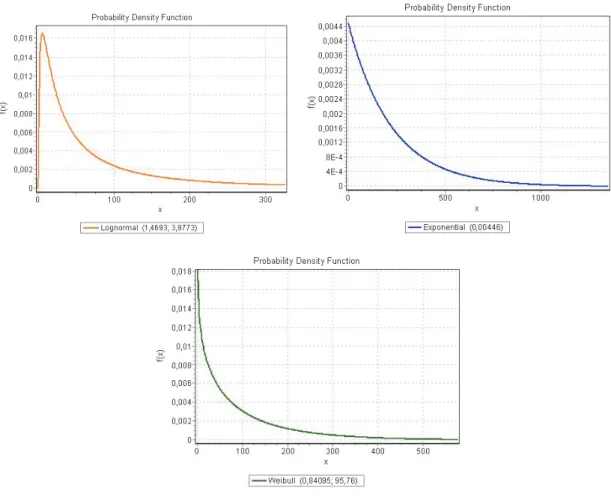
Severity, instead the frequency, is a continuous phenomenon that indicates the amount of operational losses. For the severity distribution the most common candidates are the Exponential distribution which offers the advantage of being simple (with just one parameter), and the Lognormal distribution1 proposed by Basel (2001a).
Although the Lognormal distribution is a widely spread probabilistic model, its application to leptokurtic scenarios could lead to the under-valuation of the tail of the aggregate loss distribution. In these sense, it is pointed out the importance of the kurtosis as a risk measure in non-Gaussian distributions (Stacey, 2008). Consequently, we must undertake a robust study of its suitability, and test it against other possible alternatives to ensure that the Standard LDA Model is the most risk sensitive.
Since there are many operational risk events of low and medium severity and few high- severity events, leading to heavy tailed distributions with excess kurtosis. This will have to determine the probability distribution that best fits the observed data.
Numerous authors have proposed different distributions for this purpose: Pareto (De Fontnouvelle, Jordan, & Rosengren, 2005), Weibull (Bocker & Kluppelberg, 2005) and Gamma distributions (Carrillo Menéndez & Suárez, 2006). Although in the fore mentioned BIS 2009 report, most of the evaluated entities used the lognormal distribution for the severity in their
1See Frachot, Moudoulaud, & Roncalli, (2003).
AMA models, we have tested a range of functions depending on the shape of the tail distribution: Exponential, Gumbel, Gamma, Lognormal, Weibull and Pareto.
There are several techniques to examine how well a sample of data adjusts a given distribution as its population. In those goodness-of-fit techniques, hypothesis test is based on measuring the discrepancy or consistency of the sample data to the hypothesized distribution.
Kolmogorov Smirnov test (K-S) is a goodness-of-fit measurement technique for one- dimensional data samples (see Chakravarti, Laha, & Roy, 1967). The results of the K-S tests are presented in Table 3:
Table 3: Goodness of fit
Distribution Parameters K-S Statistic Lognormal =1.4693 =3.8773 0.07114 Weibull =0.84095 =95.76 0.11744
Exponential =0.00446 0.40111
Pareto =0.13543 =0.03 0.4599 Gamma =0.0116 =19326.0 0.88839
From the table above, the limited degree of significance reached in the tests is emphasised.
Both the inherent nature of the operational losses and the lack of depth of the data sample, make difficult to find statistical fits with a reasonable degree of significance in practice. Although at both confidence levels its statistic is lower than the corresponding critical value, the lognormal provides with the best fit to the severity among the above distributions.
Figure 2: Potential candidates for severity
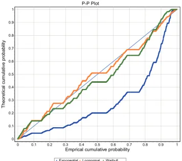
To reinforce such decision we design a probability-probability (P-P) plot and the probability difference graph. The P-P is a graph of the empirical CDF values plotted against the theoretical CDF values. It is used to determine how well a specific distribution fits to the observed data. This plot will be approximately linear if the specified theoretical distribution is the correct model. It is displayed the reference diagonal line along which the graph points should fall. According to the regulatory framework, the supervisor must validate the minimum degree of significance established by the entity for selecting the distribution of severity. In our study, we have based our decision on the value of the statistic itself. However, to support the choice of the distribution avoiding the model risk, we considered to seek further support from graphic tools such as P-P Plots (Figure 3) and the probability difference graph (Figure 4).
Figure 3: Probability-Probability (P-P) chart.
P-P Plot
Exponential Lognormal Weibull Emprical cumulative probability
1 0.9 0.8 0.7 0.6 0.5 0.4 0.3 0.2 0.1 0
Theoretical cumulative probability
1 0.9 0.8 0.7 0.6 0.5 0.4 0.3 0.2 0.1 0
Figure 4: Probability-Difference chart.
Probability Difference
Exponential Lognormal Weibull
x 60000 80000
40000 20000
0
Probability Difference
1 0.8 0.6 0.4 0.2 0 -0.2 -0.4 -0.6 -0.8 -1
The figures above illustrate the results of the tests, showing that the Lognormal distribution is the theoretical function closest to the plot of the empirical distribution, for all the cells analyzed. Consequently, this distribution has been selected for modelling the severity of operational losses, which added to the Poisson distribution give raise to the so called Standard LDA.
Aggregated Loss Distribution
In particular, for each risk type (j), in combination with a line business (i) and a given period, OR losses can be defined as a sum (Sij) of a random number (Nij) of single losses (Xij):
ijN
n ij
ij
X n
S
0
i17 , j18 (2) The actuarial model assumes2:
Single losses, Xij, are independent and identically distributed random variables.
The distribution of frequency is independent on that of the severity.
Gij is the distribution function of Sij,
0 0
0
1
x p
x x F n x pij
G
ij
n ij ij n
(3)
Where is the convolution3 operator on distribution functions and Fn is the n-fold convolution of F with itself.
Computing the aggregate loss distribution is generally not an easy task, event in the simplest cases. There are three main algorithms to calculate Gij :
Monte Carlo Method (Fishman, 1996; Klugman, Panjer, & Willmot, 2004).
Panjer’s Recursive Approach (Embrechts & Frei, 2009).
The Fast Fourier Transformation (Cooley & Tukey, 1965).
In this study we have chosen the Monte-Carlo Simulation technique to perform the convolution of both frequency and severity distributions. In particular, for each of the convolutions performed, 100,000 iterations have been generated, and relative errors considerably below 1%
have been obtained.
2See Frachot, Georges, & Roncalli (2001)
3 The mathematical convolution is a mathematical process that transforms the frequency and severity distributions in third distribution (LDA) (Feller, 1971).
Table 4: Parameter estimates for frequency and severity.
Operational Value at Risk (OpVaR)
Basel Committee on Banking Supervision defined the regulatory capital requirement (Capital-at-Risk) as follows:
“The sum of Expected Loss (EL) and Unexpected Loss (UL) for a one year holding period and a 99.9 percent confidence level, this implies that frequency distribution must be understood on a yearly basis”.
The operational risk capital requirement is evaluated through the calculation of a risk measure, like Value at Risk (VaR). It is a statistical tool that measures the worst expected loss over a specific time interval at a given confidence level. A formal definition is:
“Given some confidence level
0,1 , the VaR of a portfolio at the confidence level is given by the smallest number such that the probability that the loss L exceeds l is no
greater than (1 − ): VaR
L inf
lR|P
Ll
1
” Frequency SeveritySubwindow Subsample size Poisson Lognormal
1 6479 17,75 =1,4693 =3,8773
2 6505 17,82 =1,4693 =3,8773
3 6492 17,79 =1,4683 =3,8773
4 6476 17,74 =1,4657 =3,8748
5 6509 17,83 =1,4655 =3,8747
6 6540 17,92 =1,4644 =3,8737
7 6528 17,88 =1,4651 =3,8771
8 6564 17,98 =1,4654 =3,8775
9 6555 17,96 =1,4662 =3,8768
10 6536 17,91 =1,467 =3,8772
11 6525 17,88 =1,4673 =3,8782
12 6567 17,99 =1,4649 =3,8783
13 6599 18,08 =1,4646 =3,8791
14 6600 18,08 =1,4633 =3,8778
15 6601 18,08 =1,4627 =3,8766
16 6599 18,08 =1,4625 =3,878
17 6583 18,04 =1,4622 =3,8772
18 6562 17,98 =1,4629 =3,8773
19 6584 18,04 =1,4631 =3,8752
20 6604 18,09 =1,4617 =3,8731
21 6598 18,08 =1,4616 =3,8769
22 6612 18,12 =1,4632 =3,8769
23 6608 18,10 =1,4632 =3,877
24 6587 18,05 =1,4632 =3,8758
25 6572 18,01 =1,4632 =3,8758
26 6572 18,01 =1,4636 =3,878
27 6592 18,06 =1,4658 =3,8798
28 6617 18,13 =1,4663 =3,8798
29 6623 18,15 =1,466 =3,8771
30 6633 18,17 =1,4651 =3,8758
31 6615 18,12 =1,4661 =3,8738
In the spirit of a Value-at-Risk, the regulatory capital requirement CaR is the 99.9%
percentile of distribution of the aggregate loss, meaning that one expects to incur a loss higher than CaR, on average, once every 1,000 observations. The total loss of the bank is then the sum of aggregate losses for each business line and loss type class.
Thus, the regulatory capital, in the last case, to risk type j within a business line i as a confidence level
must be equal to:OpVaR CaRij ELijULij
(4) Unless the bank can demonstrate that it is adequately capturing EL in its internal business practices, in this new situation:OpVaR CaRij ULij
(5) When the LDA distribution has been determined, the OpVaR99.9% must be calculated to infer the regulatory capital.In our empirical study, we only have one line of business in the IOLD and owing to the scarcity of data, we have not classified the losses according to the type of error, we just take the sum of them as the total operational loss, so we only have to calculate one. This study has been carried out under the assumption that the credit entity has not made provision for its expected loss (EL). Consequently, the capital requirements have to cover both this loss and the unexpected loss (UL); thus we can identify the OpVaR with the amount of the Capital at Risk (CaR) using equation (4). The results obtained for the first back-testing point are shown in Table 5. In this case, the EL = 2,532.75, the OpVaR99.9% = 17,970.38. Then, we obtain, by difference, the UL = 17,970.38 - 2,532.75 = 15,437.63
Table 5: Aggregated Loss Distribution’s percentiles.
Percentiles Value 75% 3,105.36 80% 3,405.35 85% 3,796.96 90% 4,369.17 95% 5,448.11 99% 8,810.23 99.9% 17,970.38
In regulatory terms, the percentile of the distribution of aggregate losses that determines the Capital at Risk is established at 99.9%. The fact that the Committee has recommended such a high percentile has aroused criticism and a certain apprehension in the banking sector.
Given the leptokurtic character of operational losses, this percentile may lead to an overestimation of the capital required, and may even represent an unsustainable amount in the capital structure of a credit entity. However, the intention of the Committee is precisely to cover the risk of possible extreme losses located in the tail of the distribution. In order to calibrate the
impact of the percentile, we have compared the OpVaR calculated at the 99.9 percentile with that obtained by applying other less conservative percentiles, that is, 95% and 99%, which are commonly used in the determination of capital charge for market risk.
3. BACK-TESTING: BASIC ANALYSIS
In its simplest form, the back-testing procedure consists of calculating the number or percentage of times that the operational losses fall outside the OpVaR estimates, these are called exceedences or exceptions, and comparing that numbers with the confidence level used.
For example, if the confidence level were 99%, we can expect an exception every 100 days.
With too many exceptions, the model underestimates risk. This involves systematically comparing the history of OpVaR forecasts with their corresponding real losses.
As Figure 5 illustrates, we observe that the operational loss series exceeds once to OpVaR99.9%, twice to OpVaR99% and four-time OpVaR95%. These results are logical in the sense that the higher the confidence level is the more conservative measure reports and, consequently, higher capital charge is required.
Figure 5: Real Losses against different estimated OpVaRs.
0.00 € 2,000.00 € 4,000.00 € 6,000.00 € 8,000.00 € 10,000.00 € 12,000.00 € 14,000.00 € 16,000.00 € 18,000.00 € 20,000.00 €
01/1 2/2006
02/1 2/2006
03/1 2/2006
04/1 2/2006
05/1 2/2006
06/1 2/2006
07/1 2/2006
08/1 2/2006
09/1 2/2006
10/1 2/2006
11/1 2/2006
12/1 2/2006
13/1 2/2006
14/1 2/2006
15/1 2/2006
16/1 2/2006
17/1 2/2006
18/1 2/2006
19/1 2/2006
20/1 2/2006
21/1 2/2006
22/1 2/2006
23/1 2/2006
24/1 2/2006
25/1 2/2006
26/1 2/2006
27/1 2/2006
28/1 2/2006
29/1 2/2006
30/1 2/2006
31/1 2/2006
Operational Losses OpVaR95% OpVaR99% OpVaR99.9%
Figure 6: Back-testing Flowchart
Once the phase of modeling is over, some statistics test will help to compute the accuracy of the model. Basically these tests provide us knowledge of:
The frequency of violations, also called the unconditional coverage property: the likelihood of generating an excess over the reported VaR must be exactly1 , where
is the confidence level.
The clustering of the violations: This can eventually indicate that a sequence of violation can be explained for a single event or that the risk model was not able to protect against unexpected losses.
Basel II does not describe any specific procedure for back-testing the operational risk It is only stated that: “Whatever approach is used, a bank must demonstrate that its operational risk measure meets a soundness standard comparable to that of the internal ratings-based approach for credit risk, (i.e. comparable to a one year holding period and a 99.9th percentile confidence interval)”.
Operational Value at Risk
OpVaR
Back-testing (Basic Analysis )
Accept ? NO
Back-testing (Statistical Analysis )
Accept ? NO
YES
End
Kupiec Test
Christoffersen Test Binary Indicator
Extremal Index
On the contrary, there is an explicitly regulatory framework for market risk Basel II (2006, Annex10a). It is based on the number of exceptions over 250 daily observations generated by bank VaR models with a 99% confidence level. Depending on the results, the supervisor may impose a penalty corresponding to an increase in market risk capital via the scaling factor (K), the most exceptions a system has the higher the penalty is. To help supervisors interpret back-testing results, the Basel Committee introduced a three-zone framework related to the number of exceptions recorded. In this sense, the only first property mentioned above is taking into account.
Testing the Unconditional Coverage Property: The Binary Indicator (BI)
Following Cruz (2002), once calculated the OpVaR, it is necessary to determine whether the risk is being measured adequately. This test requires recursive estimates of OpVaR for a given holding period. A series of exceptions, named Binary Indicator, is constructed as:4
t t t
t t t
t
t if X OpVaR
OpVaR X
I if
| 1 1
| 1 1
|
1 0
1 (6)
This function will take the value one when actual losses are higher than estimated. Therefore, the exceptions It1|t are distributed as a Bernoulli (p), wherep1
.1. The actual total numbers of exceptions (E~
) is calculated as:
E~
=
1
| 1 n
m t
t
It (7) 2. The actual proportion of exceptions (p*) is calculated as:
p*=
m n
I
n m
t t t
1
| 1
(8) 3. The total number of expected exceptions (E) for a given confidence level is calculated as:
E = * (n-m) (9)
With these calculations we are able to decide whether to reject or not the model.
It rejects the model if E~ E, equivalently if p* p
It accepts the model if E~
< E, equivalently if p*<p
4 It is also named as hit sequence.
Testing the Independence Property: The Extremal Index (EI)
Several large loss events together may indicate a different pattern of loss events that need to be most carefully understood.
The Extremal Index (EI) is a useful and easy statistic for describing the clustering of extreme events. This index belongs to the interval [0, 1]. The closer the index is to 0 the more clustered the time series (Cruz, 2002).
To calculate the EI we will use the Block Method:
We separate the time series It1|t in blocks of a certain number of observations.
We count the number of blocks with one or more exceptions, K. And finally, we calculate:
E
EI K~ (10)
One of the advantages of estimating the EI is that it also offers alternatives to overcome a poor prediction caused a strong dependence problem, increasing the quantile used in OpVaR using the formula above:
EI
* , where
* is the new confidence level.We construct the Binary Indicator series for each confidence levels in Table 6. It shows, for the three confidence level selected, the number of times that the real operational loss exceeds the OpVaR estimate; in other words, if the Difference (Real Loss minus OpVaR) is negative, then the Binary Indicator takes the value 1, meaning that one exception has occurred.
In the first case represented in Table 6, there are 4 violations in 31 days, i.e. a 12.9%
rate of violations. The expected number of violations at 95% percentile confidence level in 31 days is 1.55. Therefore, it seems likely our basic analysis would reject the model. In all three cases p* is greater than p, therefore reject the model
Table 6: Binary Indicator for different percentiles confidence levels.
Date Operational
Losses OpVaR Difference Hit
series OpVaR Difference Hit
series OpVaR Difference Hit series 01/12/2006 3,431.92 € 5,448.11 € 2,016.19 € 0 8,810.23 € 5,378.31 € 0 17,970.38 € 14,538.46 € 0 02/12/2006 0.00 € 5,365.26 € 5,365.26 € 0 8,577.07 € 8,577.07 € 0 16,488.28 € 16,488.28 € 0 03/12/2006 0.00 € 5,473.14 € 5,473.14 € 0 8,779.11 € 8,779.11 € 0 18,353.37 € 18,353.37 € 0 04/12/2006 2,527.65 € 5,398.22 € 2,870.57 € 0 8,723.56 € 6,195.91 € 0 18,139.11 € 15,611.46 € 0 05/12/2006 6,833.89 € 5,370.18 € -1,463.71 € 1 8,552.76 € 1,718.87 € 0 16,939.45 € 10,105.56 € 0 06/12/2006 1,292.41 € 5,431.27 € 4,138.86 € 0 8,618.12 € 7,325.71 € 0 16,945.14 € 15,652.73 € 0 07/12/2006 10,822.53 € 5,428.64 € -5,393.89 € 1 8,612.85 € -2,209.68 € 1 16,035.50 € 5,212.97 € 0 08/12/2006 0.00 € 5,466.38 € 5,466.38 € 0 8,735.69 € 8,735.69 € 0 17,229.32 € 17,229.32 € 0 09/12/2006 0.00 € 5,419.42 € 5,419.42 € 0 8,625.23 € 8,625.23 € 0 16,751.06 € 16,751.06 € 0 10/12/2006 0.00 € 5,458.96 € 5,458.96 € 0 8,888.72 € 8,888.72 € 0 18,232.84 € 18,232.84 € 0 11/12/2006 7,546.77 € 5,410.57 € -2,136.20 € 1 8,660.55 € 1,113.78 € 0 16,673.30 € 9,126.53 € 0 12/12/2006 2,296.56 € 5,449.01 € 3,152.45 € 0 8,732.69 € 6,436.13 € 0 17,030.64 € 14,734.08 € 0 13/12/2006 745.47 € 5,501.86 € 4,756.39 € 0 8,735.50 € 7,990.03 € 0 16,128.77 € 15,383.30 € 0 14/12/2006 1,308.02 € 5,489.52 € 4,181.50 € 0 8,802.01 € 7,493.99 € 0 17,316.21 € 16,008.19 € 0 15/12/2006 2,739.53 € 5,439.01 € 2,699.48 € 0 8,582.24 € 5,842.71 € 0 16,405.62 € 13,666.09 € 0 16/12/2006 10.00 € 5,440.07 € 5,430.07 € 0 8,714.63 € 8,704.63 € 0 16,577.32 € 16,567.32 € 0 17/12/2006 0.00 € 5,425.97 € 5,425.97 € 0 8,602.84 € 8,602.84 € 0 16,621.82 € 16,621.82 € 0 18/12/2006 2,880.35 € 5,415.79 € 2,535.44 € 0 8,562.23 € 5,681.88 € 0 16,101.74 € 13,221.39 € 0 19/12/2006 884.34 € 5,475.23 € 4,590.89 € 0 8,697.07 € 7,812.73 € 0 16,866.40 € 15,982.06 € 0 20/12/2006 893.06 € 5,453.03 € 4,559.97 € 0 8,771.58 € 7,878.52 € 0 16,989.07 € 16,096.01 € 0 21/12/2006 5,028.33 € 5,411.86 € 383.53 € 0 8,531.88 € 3,503.55 € 0 16,850.89 € 11,822.56 € 0 22/12/2006 4,286.29 € 5,449.89 € 1,163.60 € 0 8,609.18 € 4,322.89 € 0 17,776.82 € 13,490.53 € 0 23/12/2006 0.00 € 5,459.52 € 5,459.52 € 0 8,667.32 € 8,667.32 € 0 15,755.06 € 15,755.06 € 0 24/12/2006 0.00 € 5,472.67 € 5,472.67 € 0 8,631.72 € 8,631.72 € 0 16,943.15 € 16,943.15 € 0 25/12/2006 0.00 € 5,415.84 € 5,415.84 € 0 8,645.50 € 8,645.50 € 0 16,871.61 € 16,871.61 € 0 26/12/2006 4,995.57 € 5,470.56 € 474.99 € 0 8,655.75 € 3,660.18 € 0 17,553.41 € 12,557.84 € 0 27/12/2006 16,901.31 € 5,472.48 € -11,428.83 € 1 8,680.03 € -8,221.28 € 1 16,437.95 € -463.36 € 1 28/12/2006 4,819.85 € 5,486.78 € 666.93 € 0 8,712.75 € 3,892.90 € 0 16,800.99 € 11,981.14 € 0 29/12/2006 2,315.77 € 5,501.21 € 3,185.44 € 0 8,625.36 € 6,309.59 € 0 16,627.91 € 14,312.14 € 0 30/12/2006 0.00 € 5,510.73 € 5,510.73 € 0 8,586.88 € 8,586.88 € 0 15,771.63 € 15,771.63 € 0 31/12/2006 0.00 € 5,486.41 € 5,486.41 € 0 8,693.61 € 8,693.61 € 0 16,312.19 € 16,312.19 € 0
95% 99% 99.90%
Table 7: Basic Analysis to test the unconditional coverage property.
Confidence Level 95% 99% 99.9%
Excedances in the backtesting 4 2 1
Allowed Excedances 1.550 0.310 0.031
p* 0.129 0.065 0.032
p 0.050 0.010 0.001
Conclusion REJECT REJECT REJECT
Basic Analysis
It is a simple method to be applied for testing the independence of events. For convenience, the observations have been grouped in block if six events. The table below shows the results of the clustering effect for different confidence levels.
Table 8: Extremal Index to evaluate the clustering of the exceptions.
Confidence Level 95% 99% 99.9%
Extremal Index 0.75 1 1
Conclusion Some degree of clustering No clustering No clustering Extremal
Index
As noticed, for the 95% confidence level there is some degree of clustering as two out of the four events happens in the same block. In this case, the number of blocks computing
more than one exception is 3, when the total number of exceptions is 4; therefore, the Extremal Index (EI) is calculated as follows, indicating some degree of clustering.
It would be also interesting to plot the exceptions to help us to visualize the same analysis.
Figure 7 show the time series of the Binary Indicator at each confidence level.
Figure 7: Time series of the Binary Indicator for different confidence level.
TIME SERIES OF THE BINARY INDICATOR
0 1
29/11/2006 04/12/2006 09/12/2006 14/12/2006 19/12/2006 24/12/2006 29/12/2006 03/01/2007
TIME SERIES OF THE BINARY INDICATOR
0 1
29/11/2006 04/12/2006 09/12/2006 14/12/2006 19/12/2006 24/12/2006 29/12/2006 03/01/2007
TIME SERIES OF THE BINARY INDICATOR
0 1
29/11/2006 04/12/2006 09/12/2006 14/12/2006 19/12/2006 24/12/2006 29/12/2006 03/01/2007
4. BACK-TESTING: STATISTICAL ANALYSIS
The Kupiec Test
The Kupiec test is the most widely used test of back-testing VaR is a test (Kupiec, 1995), it tests the unconditional coverage. Its standard version corresponds to a test failure rate that verifies compliance with the property of unconditional coverage. It is based on the same binomially assumption of the exception as the Basel approach.
75 . 4 0
~ 3
E EI k
The null hypothesis for this test is, Ho: p = p*, this is equivalent to prove
T E~ 1
. Where T represent the numbers of back-testing points. It proves basically whether the actual number of exception is equal to the expected number of exceptions. This can formally be tested with the following statistic (Pérignon, Deng, & Wang, 2008):
E E T E E
T
UC T
E T
p E p LR
~
~
~ ~ ~ ~
1 ln 2 1
ln
2 (11)
This statistic is asymptotically distributed
2 with one degree of freedom.Table 9: Kupiec Test results.
VaR level 95% 99% 99.9%
Luc 2.894 4.172 5.040
p-valor 0.090 0.041 0.025
Conclusion REJECT REJECT REJECT
VaR level 95% 99% 99.9%
Luc 2.894 4.172 5.040
p-valor 0.090 0.041 0.025
Conclusion ACCEPT REJECT REJECT Kupiec
Test (5%) Kupiec
Test (10%)
From the table above, given a certain significance level for the test (10%), then we would reject the null hypothesis. On the contrary, for a lower significance level (5%), then we would accept the null hypothesis just only for the case of OpVaR95%.The choice of significance level comes down to an assessment of the costs of making two types of mistakes: We could reject a correct model (Type I error) or we could accept an incorrect model (Type II error). Increasing the significance level implies larger Type I errors but smaller Type II errors and vice versa. In academic work, a significance level of 1%, 5%, or 10% is typically used. In operational risk, the Type II errors may be very costly so that a significance level of 10% may be appropriate.
The Christoffersen’s Test
A well-known limitation of the unconditional coverage test is that it ignores exception clustering. (Christoffersen, 2004) develops a conditional coverage test, which formally accounts for clusters of exceptions and verifies the unconditional coverage.
It is based on the assumption that the sequences of random variables It1|t follow a Markov chain of order one.
IND UC
CC LR LR
LR (12)
Specifically, the null hypothesis in the independence test LRIND states that the likelihood of a violation on a given day does not depend on whether or not a violation occurred on the previous day, H0:
0
100 10 01 11 2ln
1 0
00 0 01
1 1
10 111
~
~ 1 ln
2 T T T T
T T T T
IND T
E T
LR E
(13)
Where Tij is the number of days in which state j occurred in one day while it was at i the previous day and
i is the probability of observing an exception conditional on state i the previous day,01 00
01
0 T T
T
and11 10 1 11
T T
T
.LRCC statistic is asymptotically distributed
2 with two degrees of freedom. It is jointly test whether the observations of It1|t are independent and if the average excess is actually close to the level of significance assumed for the model, 1
.As a practical matter, when implementing the LRind tests one may incur samples where T11 = 0. In this case, we simply calculate the likelihood function as:
10 01 11
00 ~
~ 1 ln 2
T T T T
IND T
E T
LR E (14)
Table 10: Christoffersen’s Test results.
VaR level 95% 99% 99.9%
Lcc 0.96 2.94 6.79
p-valor 0.6704 0.2232 0.0369
Conclusion ACCEPT ACCEPT REJECT
VaR level 95% 99% 99.9%
Lcc 0.96 2.94 6.79
p-valor 0.6704 0.2232 0.0369
Conclusion ACCEPT ACCEPT REJECT
Christofferesen's Test (10%)
Christofferesen's Test (5%)
For both significance levels (5% and 10%) the OpVar95% and OpVaR99% are accepted, whereas the OpVaR99.9% model is rejected.
5. CONCLUSIONS
In this paper we have conducted an empirical back-testing exercise to calibrate the accuracy of the capital charges estimates (OpVaR) for covering operational risk, by using an advanced methodology such as the Loss Distribution Approach (LDA). In short, the back-testing analysis compares the operational losses experienced by a financial institution with the OpVaR previously estimated. Although this complementary exercise might be simple from a conceptual point of view, in practice, the computational calculation required to calculate daily OpVaRs on the LDA basis is tedious and time consuming. Firstly; both the frequency and the severity of operational losses should be characterized by estimating the probability functions that better fits the data; secondly, we run 100,000 iterations for carrying out the convolution process by using the Monte Carlo simulation technique to obtain the aggregated loss distribution and the corresponding 99.9 percentile; finally, this process has to be repeated 31 times to estimate the daily OpVaRs before comparing them against the real operational losses.
Our empirical results, based on the Basic Analysis, bring into light that, for the three confidence levels used (95%, 99% and 99.9%), the coverage property is not satisfied. On the contrary, the independence among the exceptions is not rejected.
On the other hand, the implications for the choice of the confidence level for the OpVaR estimates is that the larger the confidence level, the fewer the number of exceptions are permitted and therefore it will more difficult to validate the model. At 95% level it is expectable to obtain more violations than for 99%, giving rise to better test of the model accuracy. In the case of the savings bank analyzed, the 99.9% suggested by Basel II is too conservative in terms of capital charges in comparison to Market VaR, established at 99%.
One of the main problems facing the operational risk measurement is the lack of data, which affects the parameter estimates of the marginal distributions of the losses. The principal reason is that financial institutions started to collect operational loss data a few years ago, due to the relatively recent definition of this type of risk. Most banks’ internal data collection processes are still in their infancy, and there are not enough data available (especially on those rare, high-impact losses) to estimate unexpected losses.
The use of external operational loss data could be very helpful in order to supplement the current IOLD, especially for tail events, which are generally missing from internal data because of the underreporting phenomena.
6. REFERENCES
Allen, L., & Bali, T. G. (2007a). Cyclicality in catastrophic and operational risk measurements.
Journal of Banking & Finance, 31(4), 1191-1235.
Basel Committee on Banking Supervision, 2001a. Basel II: the new Basel Capital Accord Basel Committee on Banking Supervision, 2006. Basel II: International Convergence of Capital Measurement and Capital Standards: A Revised Framework. Bank for International Settlements.
Basel Committee on Banking Supervision, 2009. Observed range of practice in key elements of Advanced Measurement Approaches (AMA).
Basel Committee on Banking Supervision, 2010. Principles for enhancing corporate governance.
Bocker, K., & Kluppelberg, C. (2005). Operational VaR: A closed-form approximation. Risk- london-risk magazine limited-, 18(12), 90.
Carrillo Menéndez, S., & Suárez, A. (2006). Medición efectiva del riesgo operacional.
Estabilidad Financiera, (11), 61.
Chakravarti, I. M., Laha, R. G., & Roy, J. (1967). Handbook of methods of applied statistics:
Techniques of computation, descriptive methods and statistical inference Wiley.Chavez- Demoulin, V., Embrechts, P., & Nešlehová, J. (2006). Quantitative models for operational risk: Extremes, dependence and aggregation. Journal of Banking & Finance, 30(10), 2635- 2658.
Chernobai, A., Menn, C., Rachev, S. T., & Trûck, C. (2006). Estimation of operational value-at- risk in the presence of minimum collection thresholds. Working paper .September, Christoffersen, P. F. (2004). Back-testing and stress testing. Elements of financial risk
management (pp. 181-208). San Diego: Academic Press
Cooley, J. W., & Tukey, J. W. (1965). An algorithm for the machine calculation of complex fourier series. Mathematics of Computation, 19(90), 297-301.
Cruz, M. G. (2002). Modelling, measuring and hedging operational risk Wiley Chichester.
Cummins, J. D., Lewis, C. M., & Wei, R. (2006). The market value impact of operational loss events for US banks and insurers. Journal of Banking & Finance, 30(10), 2605-2634.
De Fontnouvelle, P., Jordan, J. S., & Rosengren, E. S. (2005). Implications of alternative operational risk modeling techniques. NBER Working Paper,
Degen, M., Embrechts, P., & Lambrigger, D. D. (2007). The quantitative modelling of operational risk: Between g-and-h and EVT. Astin Bulletin, 37(2), 265.
Dutta, K., & Perry, J. A tale of tails: An empirical analysis of loss distribution models for estimating operational risk capital. FRB of Boston Working Paper No. 06-13
Embrechts, P., & Frei, M. (2009). Panjer recursion versus FFT for compound distributions.
Mathematical Methods of Operations Research, 69(3), 497-508.
Feller, W. (1971). An introduction to probability theory and its applications, vol. 2, 2nd Ed.
Fishman, G. S. (1996). Monte carlo: Concepts, algorithms, and applications Springer.
Frachot, A., Georges, P., & Roncalli, T. (2001). Loss distribution approach for operational risk.
Frachot, A., Moudoulaud, O., & Roncalli, T. (2003). Loss distribution approach in practice. The Basel Handbook: A Guide for Financial Practioners,
Hoaglin, D. C., Mosteller, F., & Tukey, J. W. (1983). Understanding robust and exploratory data analysis Wiley New York.
Klugman, S. A., Panjer, H. H., & Willmot, G. E. (2004). Loss models: From data to decisions 2º Edition John Wiley & Sons.
Kupiec, P. H. (1995). Techniques for verifying the accuracy of risk measurement models. The Journal of Derivatives, 3(2), 73-84.
Moscadelli, M. (2004). The modelling of operational risk: Experience with the analysis of the data collected by the Basel Committee.
Stacey, J. (2008). Multi-dimensional risk and mean-kurtosis portfolio optimization. Journal of Financial Management and Analysis, 21(2)
Tukey, J. W. (1977). Exploratory data analysis. Addison-Wesley.
F
UNDACIÓN DE LASC
AJAS DEA
HORROS DOCUMENTOS DE TRABAJOÚltimos números publicados
159/2000 Participación privada en la construcción y explotación de carreteras de peaje Ginés de Rus, Manuel Romero y Lourdes Trujillo
160/2000 Errores y posibles soluciones en la aplicación del Value at Risk Mariano González Sánchez
161/2000 Tax neutrality on saving assets. The spahish case before and after the tax reform Cristina Ruza y de Paz-Curbera
162/2000 Private rates of return to human capital in Spain: new evidence F. Barceinas, J. Oliver-Alonso, J.L. Raymond y J.L. Roig-Sabaté 163/2000 El control interno del riesgo. Una propuesta de sistema de límites
riesgo neutral
Mariano González Sánchez
164/2001 La evolución de las políticas de gasto de las Administraciones Públicas en los años 90 Alfonso Utrilla de la Hoz y Carmen Pérez Esparrells
165/2001 Bank cost efficiency and output specification Emili Tortosa-Ausina
166/2001 Recent trends in Spanish income distribution: A robust picture of falling income inequality Josep Oliver-Alonso, Xavier Ramos y José Luis Raymond-Bara
167/2001 Efectos redistributivos y sobre el bienestar social del tratamiento de las cargas familiares en el nuevo IRPF
Nuria Badenes Plá, Julio López Laborda, Jorge Onrubia Fernández
168/2001 The Effects of Bank Debt on Financial Structure of Small and Medium Firms in some Euro- pean Countries
Mónica Melle-Hernández
169/2001 La política de cohesión de la UE ampliada: la perspectiva de España Ismael Sanz Labrador
170/2002 Riesgo de liquidez de Mercado Mariano González Sánchez
171/2002 Los costes de administración para el afiliado en los sistemas de pensiones basados en cuentas de capitalización individual: medida y comparación internacional.
José Enrique Devesa Carpio, Rosa Rodríguez Barrera, Carlos Vidal Meliá
172/2002 La encuesta continua de presupuestos familiares (1985-1996): descripción, representatividad y propuestas de metodología para la explotación de la información de los ingresos y el gasto.
Llorenc Pou, Joaquín Alegre
173/2002 Modelos paramétricos y no paramétricos en problemas de concesión de tarjetas de credito.
Rosa Puertas, María Bonilla, Ignacio Olmeda
174/2002 Mercado único, comercio intra-industrial y costes de ajuste en las manufacturas españolas.
José Vicente Blanes Cristóbal
175/2003 La Administración tributaria en España. Un análisis de la gestión a través de los ingresos y de los gastos.
Juan de Dios Jiménez Aguilera, Pedro Enrique Barrilao González 176/2003 The Falling Share of Cash Payments in Spain.
Santiago Carbó Valverde, Rafael López del Paso, David B. Humphrey Publicado en “Moneda y Crédito” nº 217, pags. 167-189.
177/2003 Effects of ATMs and Electronic Payments on Banking Costs: The Spanish Case.
Santiago Carbó Valverde, Rafael López del Paso, David B. Humphrey
178/2003 Factors explaining the interest margin in the banking sectors of the European Union.
Joaquín Maudos y Juan Fernández Guevara
179/2003 Los planes de stock options para directivos y consejeros y su valoración por el mercado de valores en España.
Mónica Melle Hernández
180/2003 Ownership and Performance in Europe and US Banking – A comparison of Commercial, Co- operative & Savings Banks.
Yener Altunbas, Santiago Carbó y Phil Molyneux
181/2003 The Euro effect on the integration of the European stock markets.
Mónica Melle Hernández
182/2004 In search of complementarity in the innovation strategy: international R&D and external knowledge acquisition.
Bruno Cassiman, Reinhilde Veugelers
183/2004 Fijación de precios en el sector público: una aplicación para el servicio municipal de sumi- nistro de agua.
Mª Ángeles García Valiñas
184/2004 Estimación de la economía sumergida es España: un modelo estructural de variables latentes.
Ángel Alañón Pardo, Miguel Gómez de Antonio
185/2004 Causas políticas y consecuencias sociales de la corrupción.
Joan Oriol Prats Cabrera
186/2004 Loan bankers’ decisions and sensitivity to the audit report using the belief revision model.
Andrés Guiral Contreras and José A. Gonzalo Angulo
187/2004 El modelo de Black, Derman y Toy en la práctica. Aplicación al mercado español.
Marta Tolentino García-Abadillo y Antonio Díaz Pérez 188/2004 Does market competition make banks perform well?.
Mónica Melle
189/2004 Efficiency differences among banks: external, technical, internal, and managerial Santiago Carbó Valverde, David B. Humphrey y Rafael López del Paso