Furthermore, as the transfer terms become essential again, they are weakly imposed, giving traces of the porous medium pressure and fluid velocity at the interface as coupled Lagrange multipliers. Chapter 3 describes a slight modification of the generalized Babuˇska-Brezzi theory developed in [17].
Preliminary notations
The model problem
Further notations
The augmented fully-mixed variational formulation
In the rest of the thesis, and for the sake of easier analysis, we use one that leads to the double saddle point structure. In order to prove the main theorem about the solvability of the continuous formulation (3.2), we must remember the following auxiliary result from [17].. i) Ab1 : Xb1 → Xb10 is Lipschitz continuous and strongly monotone, i.e. there exist constants γ,b α >b 0 , so that.
The discrete setting
It follows analogously to the proof of Theorem 3.1 by adapting the proof of [17, Theorem 3.1]. THE DISCRETE SETTING 25 The rest of the proof also makes use of the discrete version of Lemma 3.1. On the other hand, the linear version of theorem 3.3 is established as follows.. ii) The conditions iii) - v) from theorem 3.3 are satisfied.
It is important to note now that, from the point of view of the stability of the Galerkin schemes, it should really be required that in Theorems 3.3 and 3.4 all constants αh,γh, β1,h, andβh, and thus Chin (3.20 ) and ( 3.22), are independent of h. Needless to say, the derivation of these uniform bounds (equivalently, obtaining constants that do not depend on the mesh sizeh) becomes precisely the core issue of the numerical analysis of a given Galerkin scheme of the form (3.18). Moreover, assuming for a moment the conditions iii) - v) of Theorem 3.3 with constants independent of h, and again bearing in mind Lemma 3.2, we deduce that DP(~s)( , ) satisfies the hypotheses of the linear version given by Theorem 3.4 with also hand independent constants.
We now return to the extended fully mixed variational formulation introduced in Section 2.4 and apply Theorem 3.1 to prove that (2.34) is well placed. THE INF-SUP CONDITIONS 31Lemma 2.1], which is actually the key result using the Gˆateaux derivation of A1S.
The inf-sup conditions
Analogous to the proof of Lemma 4.2, and due to the structure of B(cf. 2.31)), we find that (4.11) corresponds to the following three independent inequalities. In fact, except for the term (τS,ηS)S appearing in (4.12), the statement of the present lemma coincides with that stated in [25, Lemma 3.6].
The main result
Thanks to the analysis developed in this chapter, the proof follows from a direct application of Theorem 3.1. It basically follows by applying backward integration of parts in (2.34) and using appropriate test functions. In this chapter, we introduce the Galerkin problem scheme (2.34) and analyze its well-posedness by establishing appropriate assumptions about the finite element subspaces involved.
MAIN RESULTS 36 In addition, to treat the mean value condition for the Darcy pressure pD, we need.
The main results
Xh×Mh if and only if there exist βeS, βeD,βeΣ > 0, independent of time, such that sup. On the other hand, we now look at the discrete kernel of B, which is defined by Vh. Then, applying the same diagonal argument used in the proof of Lemma 4.2 (see also [25, Lemma 3.8]), we find that B1 satisfies the discrete inf-sup condition uniformly on Xe1,h×Mf1,h if and only if there exists βbS ,βbD>0, independent of time, such that.
Moreover, the characterization of the elements ΛS0,h(Σ) gives the supremum in (5.13) to remain unchanged if He0,h(ΩS) is taken instead. Therefore, we can prove that the assumptions required by Theorem 3.3 are fulfilled. We begin with the following lemma, which gives hypothesis i) of this theorem and assumption (3.26) (cf. 5.18). Furthermore, suppose that the parameter ρ lies in .
On the other hand, just as for the continuous case, the discrete strong monotonicity (5.19) follows from the corresponding property of the operator A1S|. The analysis is continued with the discrete inf-sup conditions for B1 and B (cf. iv) and v) in theorem 3.3).
Particular choices of finite element subspaces
PEERS + Raviart-Thomas in 2D
SPECIAL CHOICES OF SUBSPACES OF FINITE ELEMENTS 42 Note that the product space Hh(ΩS)×Lh(ΩS)×L2h(ΩS), with Hh(ΩS) and Lh(ΩS) defined according to (5.2), initially consists of the classical PEERS introduced in [1] for a mixed finite element approximation of the linear elasticity problem with Dirichlet boundary conditions (see also [33]). In turn, Hh(ΩD)×Lh(ΩD) is the lowest-order Raviart-Thomas stable element for the mixed formulation of the Poisson problem (see, e.g. These facts are particularly important for the rest of the analysis, since, as we will Below explain that all the discrete inf-sup conditions required in the hypotheses stated in Section 5.2 are already available in the literature or can be derived from related results stated there.
Then, in order to define the spaces on the interface Σ and thereby complete the list in (5.1), we follow the simplest approach proposed in [25] and [35]. Note that (5.27) actually corresponds to a PEERS-based mixed finite element approximation of a particular linear elasticity problem in ΩS (see e.g. 4.10)) with a homogeneous Dirichlet boundary condition on ΓS and a Neumann boundary condition given by φhon Σ. Moreover, since the latter was already proved in [25, lemma 5.2], in this way we complete the complete verification of the hypothesis (H.3).
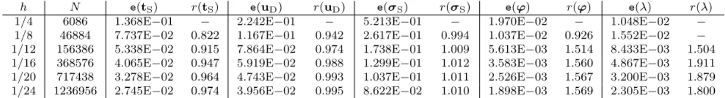
The following theorem provides the theoretical rate of convergence of the Galerkin scheme (5.5), under suitable regularity assumptions about the exact solution. The rest of the proof follows from the Cea estimate (5.31), the approximation properties of the relevant subspaces (see e.g. [4], [7] and [29]), and the fact that, thanks to the trace theorems in ΩS and ΩD, respectively, there is money.
PEERS + Raviart-Thomas in 3D
In this case, the 3D analogue of [35, Theorem 5.1], which is still an open problem, cannot be used. Therefore, to construct the stable discrete lifting of the normal traces of He0,h(ΩD) and prove the well-posed nature of the Galerkin scheme (5.27), we need to apply some inverse inequalities on Σ which require quasi-uniformity. mesh in a quarter of this interface. SPECIAL CHOICES OF FINITE ELEMENT SUBSPACES 48 discrete solutions, such that when the pair (hΣ,bhΣ) verifies hΣ ≤ C0bhΣ, it holds.
AFW + BDM in 3D
In this section, we restrict ourselves to the two-dimensional case and derive a robust and efficient residual-based estimate of the a-posterior error for our mixed finite element scheme (5.5) with discrete spaces introduced in Section 5.3.1. Most of the analyzes used in the proofs make extensive use of the estimates obtained in [22] and [26]. Therefore, as a consequence of the continuous dependence result provided by Theorem 3.2 (cf. 3.16), we conclude that the linear operator obtained by summing the two left-hand side equations (2.34), after replacing A1 with DA1(r ), satisfies the global condition inf- sup.
Moreover, thanks to the mean value theorem applied to the continuous operator A1, there exists a convex combination of tand th, say ˜s∈X1, such that. RELIABILITY OF THE POSITOR ERROR ESTIMATOR 52 where, according to (6.5) and (2.34), the residual operatorR :X×M→R is given by. 6.8) Throughout the rest of the section we provide appropriate upper bounds for each of the terms on the right-hand side of (6.8). More precisely, one proceeds as in [26] using integration by parts on each element of the triangles, using continuous and discrete Helmholtz decompositions of H(div; ΩS) and H0 (div; ΩD), and applying the Properties of the approximation of the Cl´ement and Raviart-Thomas interpolation operators in both fields (cf.
In this way and as a consequence of the analysis developed in [26], we conclude that the estimate for kRe1kH(div;Ω . S)0 is obtained from [26, Lemma 3.8] after replacing σdS,h there with tS, h +γS, h, while the estimate for kR2kH. Finally, to evaluate the remaining norms appearing on the right-hand side of (6.8), we simply use the Cauchy-Schwarz inequality and the fact that R8 can be redefined as .
Efficiency of the a posteriori error estimator
EFFECTIVENESS OF THE A POSTERIORI ERROR ROOM 57 Lemma 6.8 There exists C >0, independent of h, such that for each ∈ E(Σ) holds. Actually, it will be the only one with this property in the efficiency analysis of the terms defining ΘS,T. EFFECTIVENESS OF THE A POSTERIORI ERROR ROOM 58 Lemma 6.11 There exists C > 0, independent of h, such that for every e ∈ Eh(Σ) holds.
Similar to Lemma 6.10, we now assume an additional regularity assumption for λ to derive a local upper bound instead of the previous estimate. We begin this chapter by noting that although the decomposition (2.21) was necessary for the analysis of the continuous and discrete formulations, the actual implementation of the latter can be avoided. 7.2) Furthermore, the mean value condition required by the elements in L0,h(ΩD) can certainly be imposed by an appropriate discrete Lagrange multiplier. In the remainder of the chapter, we present numerical examples illustrating the operation of the discrete system, which validate the reliability and efficiency of the posterior error estimator Θ derived in Chapter 6, and demonstrate the behavior of the associated adaptive algorithm.
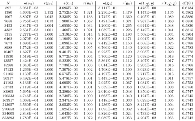
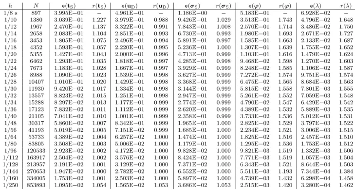
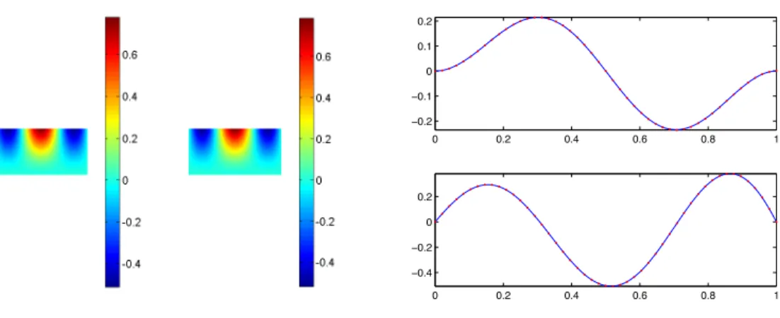
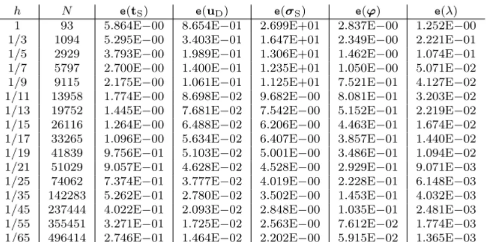
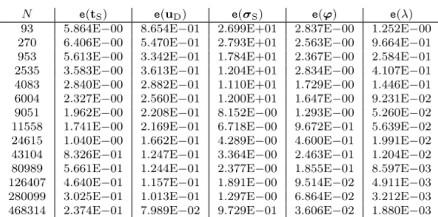
Some components of the approximate (left) and exact (right) solutions for Case 1, illustrating the accuracy of the mixed finite element scheme, are shown in Figures 7.1 and 7.2. We observe that the errors of the adaptive procedure decrease faster than those obtained with the quasi-uniform one, which is confirmed by the global experimental convergence rates reported there. From there, we conclude that the method is able to identify the origin as a singularity of the solution of this case.
Finally, some components of the approximate (left) and exact (right) solutions for case 3 are shown in Figures 7.5 and 7.6.

Trabajo futuro
In: The Mathematical Foundations of the Finite Element Method with Applications to Partial Differential Equations, A.K. Ruiz-Gal'an, A posteriori error analysis of twofold saddle point variation formulations for nonlinear boundary value problems. Meddahi, A coupled mixed finite element method for the interaction problem between an electromagnetic field and an elastic body.
Meddahi, A new doubly mixed finite element method for the plane linear elasticity problem with pure traction boundary conditions. S´anchez, A priori and a posteriori error analysis of velocity and pseudostress formulation for a class of quasi-Newtonian Stokes flows. Rudolph, A priori and a posteriori error analyzes of extended double-saddle formulations for nonlinear elasticity problems.
Oyarz´ua, A suitable mixed finite element method for coupling fluid flow with porous media flow. Sayas, A double saddle point approach for coupling fluid flow to nonlinear porous media flow.