Next, we introduce an HDG method for the gradient-velocity-pressure formulation of the Brinkman problem. A posteriori error estimates to control the L2 error of the scalar variable can be found in [20, 100]. In the context of the convection-dominated diffusion equation, [23] proposed a reliable and locally efficient residual-based error estimator for the HDG method presented in [62] , which controls the error measured in an energy norm.
3 variational formulation which makes it possible to directly relate the error in terms of residuals. In addition, all constants in the estimates are written explicitly in terms of the physical parameters α and ν. First, we recall the approximation properties of the Clément interpolation operator Ch :L1(Ω) → Vh1,c∩H01(Ω), introduced in [26], as.
Introduction
In this chapter, we propose a new technique to solve elliptic problems involving a non-polygonal interface/boundary, to develop a high-order method based on a trigonometry of the domain involving only straight elements are. As we will discuss, the boundary/interface must be interpolated by a piecewise linear function to obtain the expected convergence rates.
Boundary value problem with mixed boundary conditions
- The HDG method
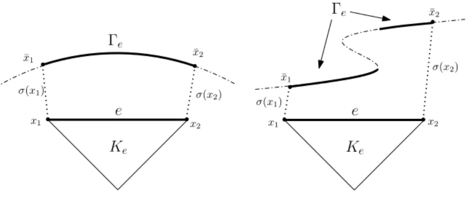
- Definition of the family of paths
- Approximation of the Neumann boundary condition
- Numerical results: Boundary-value problem
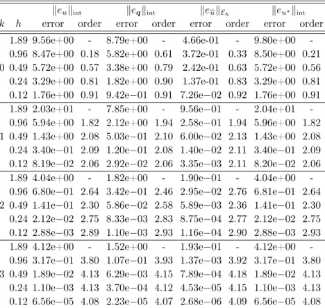
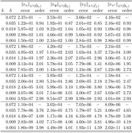
A detailed construction of the segments σ(xi) satisfying the above requirements can be found in section 2.4.2 of [41]. In this section, we present numerical experiments showing the performance of the technique proposed in previous sections and the influence of the choice of paths. Since the size of the compute domain also changes, we measure the errorseu :=u−uh,eq :=q−qhande.
The behavior of the L2 norm of the error shown in Table 1.2 corresponds to that obtained in the previous example, i.e. the rate of convergence of the error in all the variables is of order k+1. The construction of the family of paths according to (P1) in examples 1.2.1 and 1.2.2 gives similar results, since the difference between (P1) and (P2) is not significant for these domains. Indeed, for the Dirichlet problem [37] showed error estimates where some of the constants depend on the degree of the polynomial.
We point out that part of the computational domain is outside Ω, as can be observed in the inner circle in Fig. Now we test the performance of the method where Ω is a bounded domain external to an airfoil. Neumann boundary conditions are imposed around the airfoil and Dirichlet data in the remainder of the boundary.
We set f and g such that u(x, y) = sin(x) sin(y) is the exact solution as in the previous example.. Table 1.5: Convergence history of the approximation in example 1.2.5a) (solution of quiet ). In figure 1.9 we show the approximation of the x component of q taking into account 0.143 and 0.024 and k= 0.1 and 2. keukint keckkint ke . bukEh keu∗kint k h error order error order error order error order.
Elliptic interface problem
- Approximation s h D
- Imposition of s N
- Numerical results: Interface problem
- An HDG method for the Brinkman problem
- Local postprocessing of the vector solution
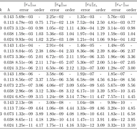
To define the approximate HD, we use the same transfer technique used for the Dirichlet data on a curved boundary (1.3). Since the computational domains Ω1h and Ω2h do not exactly fit Ω1 and Ω2, we exclude the triangles intersecting the interface from the calculation of the errors. As with the Neumann boundary data examples, the order of convergence for u and q is optimal, while the convergence of the numeric trace is suboptimal, i.e. O(hk+1).
Moreover, although superconvergence of the postprocessed solution u∗h is lost, it provides a more accurate approximation of u. In this chapter, we present an a priori error analysis for an HDG method applied to the Brinkman problem, showing optimal order of convergence of the error. We also introduce an a posteriori error estimator of the residual type, which helps us improve the quality of the numerical solution.
We establish the reliability and local efficiency of our estimator for the L2-error of the velocity and pressure gradient and the H1-error of the velocity, with constants written explicitly in terms of physical parameters and independent of grid size. We consider the Brinkman equation of incompressible flow through a porous medium under the action of an external body force and with a prescribed velocity at the boundary of the porous medium. It was motivated by the calculation of the viscous force exerted by a flowing fluid on a dense swarm of particles, where the model includes the viscous effect to determine the balance between the forces acting on the fluid volume, i.e. by the pressure gradient and the damping of the forces, αu, caused by the porous mass.
The application of the Brinkman equation derives, for example, from the composite. manufacturing [71], heat pipes [80], fuel cell computational dynamics [85] and groundwater/oil reservoir modeling. One of the features of the HDG method is the construction of an element-wise local postprocessing u∗h ofuh that approximates with higher accuracy.
A priori error analysis
We have kΠPp−ph−ΠPp−phk0,Th νkΠGL−Lk0,Th, where q is the average of q over Ω.
A posteriori error analysis
A posteriori error estimator
Here we recall that θK and θe were defined in Lemma 2.3.1 and u∗h is the post-processed solution constructed in (2.4). Note that the three volumetric terms are residues associated with the equilibrium equation, the constitutive equation, and the incompressibility condition. At the same time, the jumps over the surfaces allude to the continuity of the trace u and the normal trace νL−pI, in the case of sufficient regularity of the federal solution.
The last term, which is not common in a posteriori error estimates for Dirichlet problems, is a measure of the quality of approximation of the boundary condition. We will see that our estimator converges to zero with order min{`L, `u, `σ}+ 1 and, if L, u and pha have sufficient regularity, with order k+ 1. We begin by presenting two lemmas that they will enable us to prove the reliability of our appraiser.
So, using integration by parts and breaking the resulting boundary integral into face integrals, we arrive at After integrating the third and fourth terms of the previous expression by parts and using the fact that L =∇u, we write νkL−Lhk20,T. The next four lemmas give us the tools to prove local efficiency of our estimator.
For the rest of the proof we refer to Lemma 3.4 in [45], adapted to vector-valued functions.
The main results
Numerical experiments
- A polynomial solution
- The Kovasznay flow
- A singularly perturbed problem
- The lid-driven cavity problem
- An HDG method for the Oseen problem
- Local postprocessing of the velocity
Table 2.1 shows the history of convergence of the error for each variable when the number of elements N is quadrupled, i.e. the mesh size h decreases by a factor of two. As Tables 2.3-2.4 show, similar conclusions can be drawn regarding the optimal order of convergence of the error and the estimator. This is natural to expect, since some of the constants on the estimates depend on k.
On the other hand, we notice in all cases that the first term of the estimator (η1) is greater than the other terms. Since the solution is smooth, we can see that the curves associated with the uniform and adaptive refinements exhibit the same order of convergence predicted by theory, i.e., order N−(k+1)/2. Note that two singularities arise at the top corners of the domain, due to discontinuities in the boundary condition.
We also note that the number of elements of the adjusted mesh does not change significantly, even when we use different values of τ. We consider the Oseen equations of a viscous and incompressible fluid at small Reynolds numbers under the action of an external body force and with prescribed velocity on the boundary of the volume it contains. In fact, one of the most common approaches to approaching the solution of the incompressible Navier–Stokes equations is to consider Picard's iteration, which consists of solving Oseen equations at each step, where the convective velocity, which is divergence free, is nothing but the velocity of the previous iteration.
Since β is divergence free, it is not possible to use the standard energy argument to bound the L2 norm of the error of u and this is why a duality argument is used [51]. To complete the definition of the scheme, we specify the numerical trace νLbhn−(u\h⊗β)n−pbhn:=νLhn−(ubh⊗β)n−phn−ντ(uh−ubh)on ∂Th, where τ is a positive stabilization function on ∂Th that satisfies.

A posteriori error analysis
A posteriori error estimator
However, unlike Brinkman equations, the L2 error for the scalar variable in our case cannot be obtained directly from the formulation. This is why we use the weighted function technique used by [23] in conjunction with the convection-diffusion equations. We start by introducing three lemmas that will allow us to prove the reliability of the error estimator.
The properties of the Clément interpolant in Lemma 3.2.1 and the regularity of the mesh imply (p−ph,∇ w)Th. Now to derive an estimate for the L2 error from velocity, we proceed as in defining the auxiliary weighted function. The definition of χ will be used as an intermediate step in the proof of Lemma 3.2.4.
A posteriori error analysis 57 To bound the second term on the right-hand side, we use Cauchy-Schwarz and Young's inequalities to obtain, for any δ >0, that. Thanks to Cauchy-Schwarz and Young's inequalities, the stability and approximation properties of the Clément interpolant, the approximation property of P0 and the regularity of the family of meshes, we get that. Then, Lemmas 3.4 and 3.5 in [45] imply, adapted to vector-valued functions and considering the approximate velocity instead of its postprocessing.
The main results
Numerical experiments
- A smooth solution
- A low regularity solution
- The lid-driven cavity problem
- An application to incompressible Navier–Stokes equations
We have prepared an a posteriori error analysis for an HDG method applied to the Oseen problem. As a natural extension of the third chapter of this thesis, we are interested in proposing an a posteriori error estimator for the gradient-velocity-pressure formulation of the Navier-Stokes problem. Fully computable error bounds for discontinuous Galerkin finite element approximations on meshes with any number of levels of pendant nodes.
An a posteriori error estimate for the local discontinuous Galerkin method applied to linear and nonlinear diffusion problems. A posteriori error estimator based on gradient recovery by averaging for convection-diffusion-reaction problems, approximated by discontinuous Galerkin methods. Algebraic and discretization error estimation by equilibrium fluxes for discontinuous Galerkin methods on non-matching grids.J.
A priori and a posteriori error analyzes of an augmented HDG method for a class of quasi-Newtonian Stokes flows. A hybridizable discontinuous Galerkin method for the Navier-Stokes equations with pointwise divergence-free velocity field.
History of convergence of the approximation in Example 1.2.1
History of convergence of the approximation in Example .2
History of convergence of the approximation in Example 1.2.3
History of convergence of the approximation in Example 1.2.4
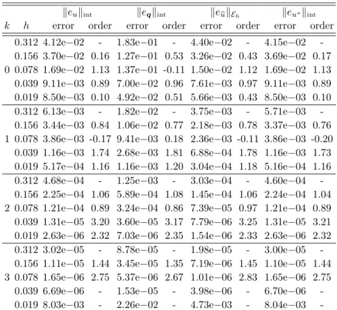
History of convergence of the approximation in Example 1.2.5a) (smooth solution)
History of convergence of the approximation in Example 1.2.5b) (non-smooth solution). 25
History of convergence of the approximation in Example 1.3.2 (kidney-shaped)
History of convergence of the approximation in Example 1.3.3 (thermal conductivity). 31
History of convergence of the terms composing the error estimator for the Example 2.4.1
History of convergence of the terms composing the error estimator for the Example .1
History of convergence of the modified global error and estimator for the Example 2.4.1
History of convergence of the terms composing the error estimator for the Example 3.3.1
History of convergence of the terms composing the error estimator for the Example 3.3.1