biosensors
Review
Trends in the Design of Intensity-Based Optical Fiber Biosensors (2010–2020)
Nerea De Acha1, Abián B. Socorro-Leránoz1,2,3,* , César Elosúa1,2 and Ignacio R. Matías1,2
Citation: De Acha, N.; Socorro- Leránoz, A.B.; Elosúa, C.; Matías, I.R.
Trends in the Design of Intensity- Based Optical Fiber Biosensors (2010–2020).Biosensors2021,11, 197.
https://doi.org/10.3390/bios11060197
Received: 9 May 2021 Accepted: 9 June 2021 Published: 15 June 2021
Publisher’s Note:MDPI stays neutral with regard to jurisdictional claims in published maps and institutional affil- iations.
Copyright: © 2021 by the authors.
Licensee MDPI, Basel, Switzerland.
This article is an open access article distributed under the terms and conditions of the Creative Commons Attribution (CC BY) license (https://
creativecommons.org/licenses/by/
4.0/).
1 Department of Electrical, Electronic and Communication Engineering, Public University of Navarra, E-31006 Pamplona, Spain; [email protected] (N.D.A.); [email protected] (C.E.);
[email protected] (I.R.M.)
2 Institute of Smart Cities, Public University of Navarra, E-31006 Pamplona, Spain
3 Navarra Institute for Health Research (IdiSNa), Recinto de Complejo Hospitalario de Navarra, C/ Irunlarrea, 3, E-31008 Pamplona, Spain
* Correspondence: [email protected]; Tel.: +34-948-169-270
Abstract:There exists an increasing interest in monitoring low concentrations of biochemical species, as they allow the early-stage detection of illnesses or the monitoring of the environment quality. Thus, both companies and research groups are focused on the development of accurate, fast and highly sensitive biosensors. Optical fiber sensors have been widely employed for these purposes because they provide several advantages for their use in point-of-care and real-time applications. In particular, this review is focused on optical fiber biosensors based on luminescence and absorption. Apart from the key parameters that determine the performance of a sensor (limit of detection, sensibility, cross-sensibility, etc.), other features are analyzed, such as the optical fiber dimensions, the sensing set ups and the fiber functionalization. The aim of this review is to have a comprehensive insight of the different aspects that must be taken into account when working with this kind of sensors.
Keywords:biosensor; optical fiber sensors; luminescence; fluorescence; absorption; localized surface plasmon resonance
1. Introduction
In recent years, great efforts have been made to enhance our quality of life. Although most of them are devoted to the treatment or curing of severe diseases [1], their prevention and early detection are not only gaining interest among scientists [2] and companies [3], but also governments [4]. These goals involve, for instance, the real-time monitoring of water and air quality [5] or the rapid detection of biomarkers related to illnesses [6]. In order to meet these requirements, accurate, highly sensitive and fast biosensing devices have been developed using different technologies. Among them, one of the most studied during the last decades is that based on optical fiber. It offers several advantages such as biocompatibility [7], the possibility of in-situ monitoring [8] and the possibility of multiparameter sensing [9], among others. These features facilitate its utilization in point- of-care and/or real-time applications.
Optical fiber-based biosensors allow monitoring two main parameters: wavelength shifts and intensity variations [10,11]. Biosensing devices characterized by the first pa- rameter were deeply analyzed in [12]. That contribution showed the three main ways to design wavelength-based optical fiber biosensors developed during last decade, as well as the benefits of working with wavelength-shift measurements. On this occasion, authors have considered it of great interest to bring together the latest advances in the field of intensity-based optical fiber biosensors within this contribution. In this manner, readers can have a broad view of the degree of development and possible applications of optical fibers as biosensing platforms.
Well-established existing technologies, such as ELISAs, fluorescence microscopy, DNA chips or flow cytometry, seem to solve the current needs in clinical analytics. Despite
Biosensors2021,11, 197. https://doi.org/10.3390/bios11060197 https://www.mdpi.com/journal/biosensors
wavelength shifts, colorimetric techniques obtaining the results after a few minutes or strip-based detections where distinguishing the symptoms at first sight (normally by using colors) and then disposing of the active part are more easy-to-handle and more familiar to what is currently used in clinical analytics. In this sense, since intensity-based optical fiber techniques detect color changes and their use is really close to the day-by-day instru- mentation in these areas, they constitute an interesting alternative to wavelength-based techniques that should not be underestimated at all. There are still some drawbacks to solve.
For instance, the instabilities of the light source while providing the optical power can affect the assays, since they can mask an eventual enhancement of the obtained measurements.
However, this is something that can be avoided by normalizing the measurements [13].
Other parameters that can also affect the measurements are temperature, relative humidity, light coupling from the sensor to the photoreceptor or the influence of ambient light.
The implementation of intensity-based optical fiber biosensors is quite simple. As it is well-known, every biosensor owns a substrate to guide the detection phenomenon, a biore- ceptor to detect the target analyte uniquely and a biofunctionalization interface to attach the bioreceptor to the substrate. In the case of the technology presented in this contribution, the substrate is the fiber itself as a transporting waveguide. This simplifies the optical set-up a lot, since there is no need for dealing with extra material that involves, for instance, fusing fibers or depositing nanofilms onto the fibers to generate resonant phenomena. As long as the evanescent field of the optical fiber is able to reach the bioreceptor-analyte interaction, the main focus is to biofunctionalize the fiber properly and then detect the target analyte. Moreover, the employed instrumentation is simple and cost-effective. Since the measurements are taken at a specific wavelength, just a simple light source (i.e., an LED) and a photodetector centered at that wavelength are needed, no matter if the light is going to be measured using either transmission or reflection set-ups.
In view of the previous considerations, this bibliographic review will focus on those optical fiber biosensors that measure intensity variations. As it will be demonstrated, the utilization of these techniques for the detection of biomolecules is widespread [14,15], taking advantage of the improvements that optical fiber technology has experienced in the last decade. To this purpose, a first section describing the main operation principles used to detect phenomena based on intensity variations (luminescence and absorption, essentially) will be addressed. Then, the optical instrumentation and configurations that are commonly employed will be revised, going through their most relevant applications. Next, the sensors performance will be analyzed in detail in terms of their limits of detection (LOD), working ranges, sensitivities, cross-sensitivities and regeneration. This information will allow the reader to have a complete overview of the most important features of luminescence and absorption-based optical fiber biosensors, something that will be summarized in the conclusions section.
2. Intensity-Based Optical Detection Phenomena
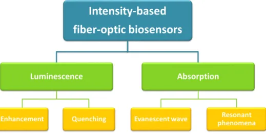
Biosensors are devices that combine specific bioreceptors (e.g., antibodies, enzymes, or DNA strands) with a transducer (in the case of this review, the optical fiber) so that the interaction between the target analyte and the bioreceptor induces a change in the measured magnitude [16]. In the case of intensity-based optical fiber sensors, that magnitude is the intensity of the light transmitted through the fiber, which can be measure using two different detection methods, mainly luminescence and absorption, which are shown in Figure1. The first one comprises those sensors based on luminescence, either when the light collected increases or decreases at a certain wavelength as a function of the analyte concentration. The second phenomenon is absorption. This will include those sensors that take advantage of the absorbing properties of the thin films deposited onto the fiber to detect what happens at a certain wavelength, or spectral range. Among the several advantages of employing thin films, the possibility of tailoring their features (selectivity, sensitivity, permeability) in the nanoscale [17], their easy fabrication and characterization [18] or
Biosensors2021,11, 197 3 of 33
the possibility of functionalizing them [19] are the most remarkable ones. They will be discussed in the corresponding section.
Biosensors 2021, 11, x FOR PEER REVIEW 3 of 34
take advantage of the absorbing properties of the thin films deposited onto the fiber to detect what happens at a certain wavelength, or spectral range. Among the several ad- vantages of employing thin films, the possibility of tailoring their features (selectivity, sensitivity, permeability) in the nanoscale [17], their easy fabrication and characterization [18] or the possibility of functionalizing them [19] are the most remarkable ones. They will be discussed in the corresponding section.
A common characteristic to every biosensor based on these techniques is the fact of working with multimode fibers. The first reason to justify this is that intensity-based sen- sors usually need a higher light intensity than phase modulated sensors [20]. In this sense, multimode fibers allow transporting high intensities along their thicker core. Moreover, it is possible to increase the light coupling by manufacturing different geometries on the optical fiber. The most representative ones are described throughout this section.
The second reason is the optical working range, since most of the reported biosensors work on the UV-VIS range. Apart from that, the use of molecular labels in the case of luminescence-based biosensors, which emit in the visible range, needs a low-loss wave- guide to where to couple and transport the luminescent emission produced.
Figure 1. Schematic of the intensity-based optical fiber biosensors analyzed in this review.
2.1. Luminescence
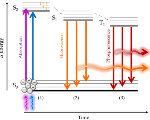
Luminescence is a well-established detection mechanism in different biomedical re- search areas. In fact, it is one of the most important sensing procedures in clinical and biological applications. It can be found when performing PCRs [21], ELISAs [22], fluores- cence microscopy [23] or gene expression in DNA chips [24], among others [25]. Its work- ing principle is based on the Jablonski’s diagram schematic shown in Figure 2. There are certain substances, called luminophores, that absorb the energy provided by photons with wavelengths located at the blue, violet and UV part of the electromagnetic spectrum. This energy is absorbed by the existing electrons in the different orbitals, which are promoted to higher energy orbitals in a process called “excitation” (1). Then, since the electrons tend to return to their lowest energy state, they will progressively go back to their original or- bitals (2), thus emitting part of the energy they have absorbed in the form of lower energy photons (3). This means at wavelengths located within the green to red and even NIR spectrum [26].
These transitions from the excited states to the ground states are called radiative tran- sitions. However, there also exist certain electron transitions where light emission does not take place. They are the non-radiative transitions (dashed arrows in Figure 2), which occur through several mechanisms, such as vibrational relaxation, intersystem crossing or internal conversion [27]. Both radiative and non-radiative transitions influence the quan- tum efficiency, this means the ratio between the absorbed photons and those emitted as luminescence. This is another important parameter that determines the behavior of a fluorophore and, therefore, its choice when performing luminescence-based measure- ments.
Figure 1.Schematic of the intensity-based optical fiber biosensors analyzed in this review.
A common characteristic to every biosensor based on these techniques is the fact of working with multimode fibers. The first reason to justify this is that intensity-based sensors usually need a higher light intensity than phase modulated sensors [20]. In this sense, multimode fibers allow transporting high intensities along their thicker core. Moreover, it is possible to increase the light coupling by manufacturing different geometries on the optical fiber. The most representative ones are described throughout this section.
The second reason is the optical working range, since most of the reported biosensors work on the UV-VIS range. Apart from that, the use of molecular labels in the case of luminescence-based biosensors, which emit in the visible range, needs a low-loss waveg- uide to where to couple and transport the luminescent emission produced.
2.1. Luminescence
Luminescence is a well-established detection mechanism in different biomedical research areas. In fact, it is one of the most important sensing procedures in clinical and biological applications. It can be found when performing PCRs [21], ELISAs [22], fluorescence microscopy [23] or gene expression in DNA chips [24], among others [25].
Its working principle is based on the Jablonski’s diagram schematic shown in Figure2.
There are certain substances, called luminophores, that absorb the energy provided by photons with wavelengths located at the blue, violet and UV part of the electromagnetic spectrum. This energy is absorbed by the existing electrons in the different orbitals, which are promoted to higher energy orbitals in a process called “excitation” (1). Then, since the electrons tend to return to their lowest energy state, they will progressively go back to their original orbitals (2), thus emitting part of the energy they have absorbed in the form of lower energy photons (3). This means at wavelengths located within the green to red and even NIR spectrum [26].
These transitions from the excited states to the ground states are called radiative transitions. However, there also exist certain electron transitions where light emission does not take place. They are the non-radiative transitions (dashed arrows in Figure2), which occur through several mechanisms, such as vibrational relaxation, intersystem crossing or internal conversion [27]. Both radiative and non-radiative transitions influence the quantum efficiency, this means the ratio between the absorbed photons and those emitted as luminescence. This is another important parameter that determines the behavior of a fluorophore and, therefore, its choice when performing luminescence-based measurements.
For radiative transitions, the duration of the emission time is known as lifetime, and it allows distinguishing between fluorescence (lifetimes from 10−10 to 10−5s) and
Biosensors2021,11, 197 4 of 33
phosphorescence (lifetimes from 10−4to 104s). The wavelength range between the emission and the absorption peaks is known as Stokes shift. The larger it is, the simpler is the experimental set-up required, as there is no need for utilizing optical filters. However, when working with continuous light sources, if both peaks are close, optical filters are necessary in order to isolate the excitation from the emission light at the photoreceptor.
For radiative transitions, the duration of the emission time is known as lifetime, and it allows distinguishing between fluorescence (lifetimes from 10
−10to 10
−5s) and phospho- rescence (lifetimes from 10
−4to 10
4s). The wavelength range between the emission and the absorption peaks is known as Stokes shift. The larger it is, the simpler is the experimental set-up required, as there is no need for utilizing optical filters. However, when working with continuous light sources, if both peaks are close, optical filters are necessary in order to isolate the excitation from the emission light at the photoreceptor.
Figure 2. Schematic of a Jablonski’s diagram showing the two kinds of luminescence.
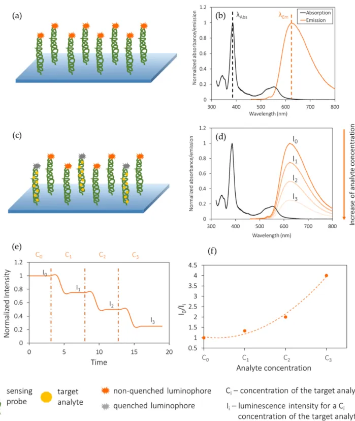
Furthermore, the luminescent intensities and lifetimes of some luminophores depend on the presence of certain analytes or on the conditions of the surrounding media [28], so they are of great interest for the development of optical biosensors. This can be done by attaching the luminophores to the bioreceptor [29,30] or to the target analyte [31]. In some cases, it is the binding between the bioreceptor and the analyte that induces changes in the surrounding medium of the luminophore [28]. This normally leads to quenching or enhancement processes (i.e., shorter or longer lifetimes). Another possibility is to label the analyte with a luminophore, so when it joins the bioreceptor, the luminescent emission can be captured. Therefore, luminescence quenching as well as luminescence enhance- ment biosensors can be developed. To the first group belong all the sensors whose inten- sity decreases in the presence of the target analyte. In the second case, the opposite phe- nomenon takes place: the luminescent emission increases due to the presence of the target analyte.
Figure 3 shows the working principle of a luminescence quenching-based optical fi- ber biosensor. The fiber is first functionalized with a luminophore-labelled bioreceptor (a) that is illuminated at the absorption wavelength of the luminophore (b). As the target analyte concentration (C
i) increases, the luminophores are quenched (c), so the emitted intensity (I
i) decreases (d). The dynamic response of the sensor is depicted in Figure 3e, whereas the obtained calibration curve is shown in Figure 3f. In the case of luminescence enhancement sensors, the opposite process occurs: as the analyte concentration increases, so does the luminescent emission. Only the first process is shown for simplicity.
Figure 2.Schematic of a Jablonski’s diagram showing the two kinds of luminescence.
Furthermore, the luminescent intensities and lifetimes of some luminophores depend on the presence of certain analytes or on the conditions of the surrounding media [28], so they are of great interest for the development of optical biosensors. This can be done by attaching the luminophores to the bioreceptor [29,30] or to the target analyte [31]. In some cases, it is the binding between the bioreceptor and the analyte that induces changes in the surrounding medium of the luminophore [28]. This normally leads to quenching or enhancement processes (i.e., shorter or longer lifetimes). Another possibility is to label the analyte with a luminophore, so when it joins the bioreceptor, the luminescent emission can be captured. Therefore, luminescence quenching as well as luminescence enhancement biosensors can be developed. To the first group belong all the sensors whose intensity decreases in the presence of the target analyte. In the second case, the opposite phenomenon takes place: the luminescent emission increases due to the presence of the target analyte.
Figure3shows the working principle of a luminescence quenching-based optical fiber biosensor. The fiber is first functionalized with a luminophore-labelled bioreceptor (a) that is illuminated at the absorption wavelength of the luminophore (b). As the target analyte concentration (Ci) increases, the luminophores are quenched (c), so the emitted intensity (Ii) decreases (d). The dynamic response of the sensor is depicted in Figure3e, whereas the obtained calibration curve is shown in Figure3f. In the case of luminescence enhancement sensors, the opposite process occurs: as the analyte concentration increases, so does the luminescent emission. Only the first process is shown for simplicity.
Biosensors2021,11, 197 5 of 33
Biosensors 2021, 11, x FOR PEER REVIEW 5 of 34
Figure 3. Working principle of a luminescence quenching-based optical fiber biosensor. (a) Fiber functionalized with a luminophore-labelled bioreceptor. (b) When illuminated at the absorption wavelength of the luminophore, luminescent emission takes place. (c) Quenching of the lumino- phore in the presence of target analyte. (d) Decrease in luminescent emission as the target analyte concentration increases. Dynamic response (e) and calibration curve (f) of the biosensor. The pur- pose of this schematic is to show the generic behavior of this kind of sensors, so the graphs do not correspond to experimental or simulated data, nor to any existing material.
As it has been explained, the luminescence emission by the luminophores occurs due the absorption of energy in the form of light, which requires their exposure to a light source. If this exposure is long-term, it can lead to a photochemical modification of the luminophore, inhibiting the transition of the electrons from the ground state to the excited ones, and, in consequence, decreasing the emitted number of photons. This phenomenon is known as photobleaching and, although it can be mathematically modeled and com- pensated [13], its effect must be reduced as much as possible because it damages the struc- ture of the luminophore [32,33].
Among the different elements that can be used as bioreceptors, aptamers (chemically synthesized DNA or RNA strands or oligonucleotides) [34], DNA strands, proteins and antibodies are the most common. Regarding the applications of these sensors, DNA [35], glucose [36] and metal ions detection [37] are the most widespread. Despite them, other bioanalytes such as proteins [38] or bacteria [30] can also be detected.
Figure 3.Working principle of a luminescence quenching-based optical fiber biosensor. (a) Fiber functionalized with a luminophore-labelled bioreceptor. (b) When illuminated at the absorption wavelength of the luminophore, luminescent emission takes place. (c) Quenching of the luminophore in the presence of target analyte. (d) Decrease in luminescent emission as the target analyte concentration increases. Dynamic response (e) and calibration curve (f) of the biosensor.
The purpose of this schematic is to show the generic behavior of this kind of sensors, so the graphs do not correspond to experimental or simulated data, nor to any existing material.
As it has been explained, the luminescence emission by the luminophores occurs due the absorption of energy in the form of light, which requires their exposure to a
light source. If this exposure is long-term, it can lead to a photochemical modification of the luminophore, inhibiting the transition of the electrons from the ground state to the excited ones, and, in consequence, decreasing the emitted number of photons. This phenomenon is known as photobleaching and, although it can be mathematically modeled and compensated [13], its effect must be reduced as much as possible because it damages the structure of the luminophore [32,33].
Among the different elements that can be used as bioreceptors, aptamers (chemically synthesized DNA or RNA strands or oligonucleotides) [34], DNA strands, proteins and antibodies are the most common. Regarding the applications of these sensors, DNA [35], glucose [36] and metal ions detection [37] are the most widespread. Despite them, other bioanalytes such as proteins [38] or bacteria [30] can also be detected.
The performance of luminescence quenching-based sensors are usually modeled by the Stern-Volmer equations, as they allow the analysis of the distribution of the lu- minophore inside the sensing film. When it is homogeneously distributed, the quencher affects the whole luminophore population equally, so the calibration curve follows a linear tendency, given by the Stern-Volmer Equation (1) [26]:
I0
I =1+KSV·[Q] (1)
where [Q] represents the concentration of the target analyte (quencher),KSVis the quench- ing constant, I0 the luminescent intensity for 0% of quencher concentration andI the luminescent intensity for a given analyte concentration.
In the cases in which the luminophore population is heterogeneously distributed, the calibration curveI0/Ifollows the Demas model [39] according to Equation (2):
I0
I =
f1
1+KSV,1·[Q]+ f2 1+KSV,2·[Q]
−1
(2) where f1and f2(f2=1−f1) correspond to the populations of the fluorophore, andKSV,1
andKSV,2to their quenching constants, respectively.
These equations are of great utility when analyzing luminescence-based systems, as they allow the investigation of bioreceptor and quencher distribution, association, diffusion and reaction at the molecular level [40].
2.2. Absorption
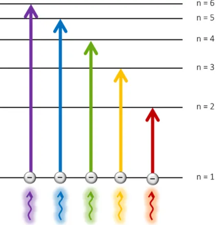
Absorption-based sensing has been commonly employed in a wide variety of ap- plications, ranging from gas detection [41] to water-quality monitoring [42], but also biodetection [43]. The transduction principle is determined by the energy levels of the dif- ferent materials: as electrons can only exist in discrete energy levels, to be moved from the ground state to higher energy levels, they must absorb enough energy, which is acquired from the absorbed light, as it is depicted in Figure4. Thus, the absorption spectrum of a certain material represents the wavelengths at which light provides to its electrons enough energy to reach higher energy levels.
There are several ways of detecting the presence of analytes using this technique.
However, it is important to classify them according to how the absorption takes place.
A first group of absorption-based sensors is that in including a selective group of sub- stances, which due to their internal structure, conformation, polarization or even their own chemistry or physics, they can absorb light at a specific wavelength. This is the case of substances such as acetone, ozone, sulfur dioxide or transition metals, which present an absorption band within the UV range [44,45]. Their detection can be carried out with no sensitive material coatings onto the substrate (i.e., the optical fiber) [46].
Biosensors2021,11, 197 7 of 33
Biosensors 2021, 11, x FOR PEER REVIEW 6 of 34
The performance of luminescence quenching-based sensors are usually modeled by the Stern-Volmer equations, as they allow the analysis of the distribution of the lumino- phore inside the sensing film. When it is homogeneously distributed, the quencher affects the whole luminophore population equally, so the calibration curve follows a linear ten- dency, given by the Stern-Volmer Equation (1) [26]:
𝐼
𝐼 1 𝐾 𝑄 (1)
where [Q] represents the concentration of the target analyte (quencher), K
SVis the quench- ing constant, I
0the luminescent intensity for 0% of quencher concentration and I the lumi- nescent intensity for a given analyte concentration.
In the cases in which the luminophore population is heterogeneously distributed, the calibration curve I
0/I follows the Demas model [39] according to Equation (2):
𝐼 𝐼
𝑓
1 𝐾
,𝑄
𝑓
1 𝐾
,𝑄 (2)
where 𝑓 and 𝑓 ( 𝑓 1 𝑓 ) correspond to the populations of the fluorophore, and 𝐾
,and 𝐾
,to their quenching constants, respectively.
These equations are of great utility when analyzing luminescence-based systems, as they allow the investigation of bioreceptor and quencher distribution, association, diffu- sion and reaction at the molecular level [40].
2.2. Absorption
Absorption-based sensing has been commonly employed in a wide variety of appli- cations, ranging from gas detection [41] to water-quality monitoring [42], but also biode- tection [43]. The transduction principle is determined by the energy levels of the different materials: as electrons can only exist in discrete energy levels, to be moved from the ground state to higher energy levels, they must absorb enough energy, which is acquired from the absorbed light, as it is depicted in Figure 4. Thus, the absorption spectrum of a certain material represents the wavelengths at which light provides to its electrons enough energy to reach higher energy levels.
Figure 4. Schematic of an absorption-based technique. Incident photons promote electrons to higher level orbitals, leading to absorption/transmission phenomena as a function of the analyte increasing concentration.
Figure 4.Schematic of an absorption-based technique. Incident photons promote electrons to higher level orbitals, leading to absorption/transmission phenomena as a function of the analyte increasing concentration.
A second group is comprised of those sensors that need the functionalization of a substrate with a bioreceptor or a sensing film onto it [47]. They are often based on evanescent wave absorption (EWA), which consists of the interaction of part of the light transmitted through the substrate with the surrounding medium [48]. Specifically, the evanescent wave is modified by changes on the refractive index of the surrounding medium, which increases or decreases the light coupled to the cladding modes of the fiber substrate.
A critical factor here is the penetration depth of the evanescent wave (dp). If dpreaches the bioreceptor-analyte area, it will be possible to detect the magnitude of the biological interaction. In this case, the presence of substances that absorb light in the range of the working wavelengths will cause a reduction in the transmitted intensity.
The last option is also based on EWA, but it has been considered apart due to the recent developments and high number of contributions recently published. In some specific cases, optical fiber structures designed to detect wavelength shifts are used as absorption-based biosensors. That is the case of Localized Plasmon Surface Resonances (LSPR) using metallic nanoparticles (NPs), usually made of gold (Au) or silver (Ag) [49]. These NPs are of great interest as they can be biofunctionalized with a specific bioreceptor to detect the target analyte [50]. In these cases, once the LSPR is located at the desired wavelength, the univocal bioreceptor—analyte interaction induces more or less absorption [12] as a function of the increasing analyte concentration, allowing the characterization of this kind of biosensors.
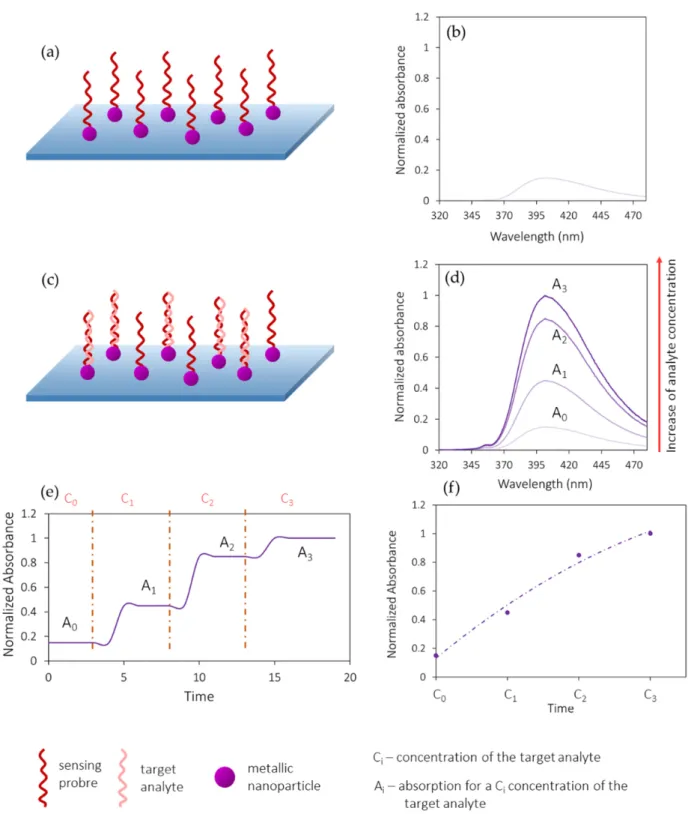
Figure5shows the working principle of an absorption-based biosensor developed using a metallic nanoparticle functionalized with a bioreceptor (a). This sensing probe presents an original absorption band centered at a determined wavelength (b). As the concentration of the target analyte increases (c), it binds the bioreceptor and this makes the absorbance increase (d), which can be taken into account to monitor the dynamic response of the biosensor as well as to obtain its calibration curve (e and f). This working principle can be applied to other absorption-based sensors that do not require a previous
functionalization of the optical fiber. In those cases, the initial absorbance will increase as a function of the analyte concentration.
Biosensors 2021, 11, x FOR PEER REVIEW 8 of 34
Figure 5. Working principle of an absorption-based optical fiber biosensor. (a) Fiber coated with a metallic nanoparticle-labelled bioreceptor. (b) Original absorption spectrum centered at a deter- mined wavelength. (c) Increasing bioreceptor—analyte binding, which increases the absorption at that wavelength (d). (e) Dynamic response and (f) calibration curve of the optical fiber biosensor.
The purpose of this schematic is to show the generic behavior of this kind of sensors, so the graphs do not correspond either to experimental or simulated data, or to any existing material.
3. Optical Parameters Analyzed
The response of an optical fiber biosensor is influenced by the optical instrumentation and also by the number of correctly attached bioreceptors to the optical substrate and their performance. Regarding the optical instrumentation, the combination of the light source, the photodetector and the optical fiber geometries should discriminate minimum intensity varia- tions, which increases the system resolution. In relation to the bioreceptors, they play a key role as they are responsible for the detection of the target analytes. An optimized combination of both of bioreceptors and instrumentation will determine the response of the optical biosen- sors, as it defines their parameters, i.e., the sensitivity, LOD, dynamic range, regeneration and cross-sensitivity. All of them are going to be analyzed in this section.
The calibration curve of an optical intensity-based biosensor is a function that pre- sents the evolution of the emitted or absorbed light by this biosensor as the analyte is progressively detected. As shown in Figure 6, after obtaining this graph it is possible to
Figure 5.Working principle of an absorption-based optical fiber biosensor. (a) Fiber coated with a metallic nanoparticle- labelled bioreceptor. (b) Original absorption spectrum centered at a determined wavelength. (c) Increasing bioreceptor—
analyte binding, which increases the absorption at that wavelength (d). (e) Dynamic response and (f) calibration curve of the optical fiber biosensor. The purpose of this schematic is to show the generic behavior of this kind of sensors, so the graphs do not correspond either to experimental or simulated data, or to any existing material.
Biosensors2021,11, 197 9 of 33
3. Optical Parameters Analyzed
The response of an optical fiber biosensor is influenced by the optical instrumentation and also by the number of correctly attached bioreceptors to the optical substrate and their performance. Regarding the optical instrumentation, the combination of the light source, the photodetector and the optical fiber geometries should discriminate minimum intensity variations, which increases the system resolution. In relation to the bioreceptors, they play a key role as they are responsible for the detection of the target analytes. An optimized combination of both of bioreceptors and instrumentation will determine the response of the optical biosensors, as it defines their parameters, i.e., the sensitivity, LOD, dynamic range, regeneration and cross-sensitivity. All of them are going to be analyzed in this section.
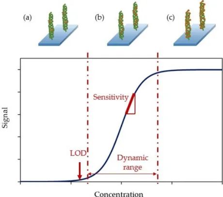
The calibration curve of an optical intensity-based biosensor is a function that presents the evolution of the emitted or absorbed light by this biosensor as the analyte is progres- sively detected. As shown in Figure6, after obtaining this grapH it is possible to deduct three main magnitudes that can describe the performance of the biosensor: the sensitivity, the LOD and the dynamic range. These three together with other interesting parameters will be analyzed below, in order to establish the different classifications that will be made in the next section.
Biosensors 2021, 11, x FOR PEER REVIEW 9 of 34
deduct three main magnitudes that can describe the performance of the biosensor: the sensitivity, the LOD and the dynamic range. These three together with other interesting parameters will be analyzed below, in order to establish the different classifications that will be made in the next section.
Figure 6. Sensitivity, limit of detection and dynamic range of a calibration curve. (a) The LOD is the minimum detectable concentration of the analyte, (b) the dynamic range is limited by the LOQ and the upper limit and (c) over the upper limit, the bioreceptor is saturated and it is not capable of detecting higher concentrations of the analyte.
• Sensitivity: it is the slope of the calibration curve. That is, the ratio between the inten- sity (or absorbance) variation and the analyte concentration variation, typically meas- ured at every point of the calibration curve. In the case of luminescence-based bio- sensors, the corresponding expression is given by (3), while for absorption-based bi- osensors, the intensity increment should be substituted by an absorption increment.
𝑆 = ∆𝐼
∆[𝑎𝑛𝑎𝑙𝑦𝑡𝑒]
(3)while intensity and absorbance are always expressed in arbitrary units (AU), the an- alyte concentrations can be expressed in different units (mol/L, colony forming units (CFU), etc.) depending on the way the analyte concentration is measured. Moreover, the responses of the sensors tend not to be linear but sigmoidal. Normally, after tak- ing the data it is typical to perform a data conditioning to logarithmic scales before calculating their sensitivities [51].
• Limit of detection (LOD): it is the lowest amount of analyte that can be detected but not necessarily quantitated by the sensor [52]. It is typically calculated as the mean of the values of the reference base line plus three times their standard deviation (4):
𝑦 = 𝑦 + 3𝜎 (4)
where 𝑦 is the LOD of the sensor, 𝑦 corresponds to the average of the refer- ence samples and 𝜎 is the standard deviation.
Figure 6.Sensitivity, limit of detection and dynamic range of a calibration curve. (a) The LOD is the minimum detectable concentration of the analyte, (b) the dynamic range is limited by the LOQ and the upper limit and (c) over the upper limit, the bioreceptor is saturated and it is not capable of detecting higher concentrations of the analyte.
• Sensitivity: it is the slope of the calibration curve. That is, the ratio between the intensity (or absorbance) variation and the analyte concentration variation, typically measured at every point of the calibration curve. In the case of luminescence-based biosensors, the corresponding expression is given by (3), while for absorption-based biosensors, the intensity increment should be substituted by an absorption increment.
S= ∆I
∆[analyte] (3)
while intensity and absorbance are always expressed in arbitrary units (AU), the analyte concentrations can be expressed in different units (mol/L, colony forming units (CFU), etc.) depending on the way the analyte concentration is measured.
Moreover, the responses of the sensors tend not to be linear but sigmoidal. Normally, after taking the data it is typical to perform a data conditioning to logarithmic scales before calculating their sensitivities [51].
• Limit of detection (LOD): it is the lowest amount of analyte that can be detected but not necessarily quantitated by the sensor [52]. It is typically calculated as the mean of the values of the reference base line plus three times their standard deviation (4):
yLOD=yblank+3σblank (4)
whereyLODis the LOD of the sensor,yblankcorresponds to the average of the reference samples andσblankis the standard deviation.
• Dynamic range: is the range of analyte concentrations between the limit of quantifica- tion (LOQ) and the upper limit. The first one is the minimum analyte concentration that can be detected and measured, while the second corresponds to the maximum concentration that the sensor can detect without being saturated.
• Cross-sensitivity: it is defined as its sensitivity towards other substances different from the target analyte [53]. As it is an indicator of the selectivity of a sensor, it is a key parameter when characterizing it.
• Resolution: it is the minimum change of the measured magnitude that can be de- tected [54].
• Detection media: apart from detecting biomolecules in standard conditions (i.e., ultrapure water or buffered solutions), biosensors should be capable of working in serum samples, real samples or, at least, solutions that mimic them.
• Regeneration: an effective manner of reducing the cost per test is the possibility of reusing the biosensors. Thus, regenerating the sensors surface has become of great interest and several mechanisms have been developed to reach this goal.
4. Classification and Discussion on Intensity-Based Optical Fiber Biosensors 4.1. Optical Fiber Biosensors Based on Luminescence
Luminescent sensors monitor the concentration of the target analyte by measuring the intensity variations of the employed luminophore. Due to the reduced dimensions of the optical fiber, light coupling from the luminophore to the photoreceptor is critical [55].
Thus, several optical schemes are employed, although the reflection architecture is the most widespread [13]. In particular, tapering the tip of the optical fiber increases the area of the sensing surface, allowing to maximize the luminescence coupling and to minimize the reflection of the excitation light [56]. On the contrary, using a transmission set-up hinders the light coupling from the fiber to the sensing film as well as from the sensing film to the photodetector. In spite of that, some authors still use that architecture [57]. The previous three sensing schemes are depicted in Figure7.
With the same goal of increasing the interaction area between the probe and the analyte, multimode fibers (made of silica or a polymeric material) are used as substrates when fabricating these sensors. The typical fiber diameters employed range from 400µm to 1.96 mm [35,58]. Lower fiber core diameters are less common, but are still used [59].
DNA detection is based on the high affinity shown by complementary DNA strands [60].
These sensors consist of the adsorption of the bioreceptor (i.e., a single-stranded DNA) which is complementary to the target DNA strand, onto the surface of the optical fiber [29,35]. For instance, Long et al. developed a biosensing platform capable of detecting 3.2 aM of the target DNA [31]: the single-stranded DNA that served as bioreceptor was immobilized onto a silanized 600µm-core tapered optical fiber using streptavidin and the heterobifunctional cross-linkerN-(4-maleimidobutyryloxy) succinimide (GMBS). The sensor was exposed to dif- ferent quantum dot (QD)-labeled DNA strands: complementary DNA, one-base mismatched complementary DNA, and non-complementary DNA. Due to the hybridization between the
Biosensors2021,11, 197 11 of 33
DNA strand and the QD-labeled complementary DNA, the fluorescence intensity increased as the concentration of the complementary DNA did (Figure8), while no fluorescent emission was detected in the presence of non-complementary DNA. Furthermore, the surface of the sensor was regenerated using sodium dodecyl sulfate (SDS) at pH 1.9, which allowed its reuse at least 30 consecutive times, with a decrease in the maximum fluorescence intensity lower than 8%.
Biosensors 2021, 11, x FOR PEER REVIEW 10 of 34
•
Dynamic range: is the range of analyte concentrations between the limit of quantifi- cation (LOQ) and the upper limit. The first one is the minimum analyte concentration that can be detected and measured, while the second corresponds to the maximum concentration that the sensor can detect without being saturated.
•
Cross-sensitivity: it is defined as its sensitivity towards other substances different from the target analyte [53]. As it is an indicator of the selectivity of a sensor, it is a key parameter when characterizing it.
•
Resolution: it is the minimum change of the measured magnitude that can be de- tected [54].
•
Detection media: apart from detecting biomolecules in standard conditions (i.e., ul- trapure water or buffered solutions), biosensors should be capable of working in se- rum samples, real samples or, at least, solutions that mimic them.
•
Regeneration: an effective manner of reducing the cost per test is the possibility of reusing the biosensors. Thus, regenerating the sensors surface has become of great interest and several mechanisms have been developed to reach this goal.
4. Classification and Discussion on Intensity-Based Optical Fiber Biosensors 4.1. Optical Fiber Biosensors Based on Luminescence
Luminescent sensors monitor the concentration of the target analyte by measuring the intensity variations of the employed luminophore. Due to the reduced dimensions of the optical fiber, light coupling from the luminophore to the photoreceptor is critical [55].
Thus, several optical schemes are employed, although the reflection architecture is the most widespread [13]. In particular, tapering the tip of the optical fiber increases the area of the sensing surface, allowing to maximize the luminescence coupling and to minimize the reflection of the excitation light [56]. On the contrary, using a transmission set-up hin- ders the light coupling from the fiber to the sensing film as well as from the sensing film to the photodetector. In spite of that, some authors still use that architecture [57]. The pre- vious three sensing schemes are depicted in Figure 7.
Figure 7. Different sensing schemes to fabricate luminescence-based optical fiber biosensors. (a) An optical fiber with a tapered tip increases its sensing surface gently (reflection architecture). (b) Figure 7.Different sensing schemes to fabricate luminescence-based optical fiber biosensors. (a) An
optical fiber with a tapered tip increases its sensing surface gently (reflection architecture). (b) A per- pendicular cut on the tip of an optical fiber is also used for biosensing using a reflection architecture.
(c) In the transmission architecture, the sensing region is located along the fiber core.
Luminescent indicators can be attached to the bioreceptor instead of to the target DNA strand. It is so in the case of Giannetti et al. [29], where the molecular beacon 50-(ATTO647N)GAGAAAGGGCTGCCA(Thiol)-30was immobilized onto a 600µm-core tapered optical fiber. The sensor was exposed to a DNA sequence complementary to that acting as bioreceptor as well as to random DNA strands: the luminescent emission increased as the presence of the target DNA did. However, no variation of the luminescent intensity was observed in the presence of random DNA sequences.
Apart from the detection of complementary DNA strands [61], the monitoring of other analytes, for instance, mercury (Hg2+) or lead (Pb2+) ions is also a widespread application of fluorophore-labeled DNA sequences [62,63]. In the first case, the detection of Hg2+ions is due to the conformational change induced by these ions into thymine(T)- rich oligonucleotide (ON) sequences: in the presence of Hg2+ions, T-Hg2+-T mismatches are formed [64], so the T-rich sequences acquire a hairpin structure [65]. Furthermore, those T-Hg2+-T base pairs quench the luminescent emission of the indicator labeled to the ON sequences [66]. For instance, the sensor described in [51] exhibited an LOD of 4.73×10⁻¹³ M Hg2+ ions in a phosphate buffered solution (pH 7.4). Due to the high affinity of Hg2+ions to T bases, the sensor responded in less than 25 s for the highest Hg2+
concentrations in a reversible manner (Figure9a), and it showed a low cross-correlation to other metallic ions (Figure9b). The sensor also allowed the measurement of 5×10⁻¹²M Hg2+ions in ultrapure and tap water.
Biosensors 2021, 11, x FOR PEER REVIEW 12 of 34
Figure 8. (a) Kinetic curves representing the molecular interactions on the sensor surface. (b) De- termination of binding kinetics for DNA hybridization. Reprinted with permission from [31].
(a)
Figure 8.(a) Kinetic curves representing the molecular interactions on the sensor surface. (b) Deter- mination of binding kinetics for DNA hybridization. Reprinted with permission from [31].
Aptamers present the advantage of being highly specific bioreceptors [67], so they are of great interest for the development of biosensors. Among many other applications, they can be employed for the detection of endocrine disrupting compounds, such as 17β- estradiol [68]. Taking advantage of this, N. Yildirim and co-workers [69] reported an optical fiber biosensor capable of detecting 17β-estradiol concentrations from 5×10⁻⁹to 75×10−9M, with a LOD of 2.1×10⁻⁹M. Its regeneration was carried out with a 0.5%
SDS solution (pH 1.9) for 90 s. Furthermore, the biosensor was not only tested in Tris-HCl buffer, but also in wastewater treatment effluent samples.
Biosensors2021,11, 197 13 of 33
Biosensors 2021, 11, x FOR PEER REVIEW 12 of 34
Figure 8. (a) Kinetic curves representing the molecular interactions on the sensor surface. (b) De-
termination of binding kinetics for DNA hybridization. Reprinted with permission from [31].
(a)
Biosensors 2021, 11, x FOR PEER REVIEW 13 of 34
(b)
Figure 9. (a) Normalized luminescence variation for 5 × 10⁻¹² M, 10−11 M, 5 × 10⁻¹¹ M, 10−10 M, 5 ×10⁻¹⁰ M, 10−9 M and 5 × 10⁻⁹ M concentrations in 10 mM PBS (pH 7.4), and regeneration with 0.5%
w/w SDS. (b) I0/I ratio of the sensor in the absence of metal ions (blank), in the presence of 10−9 M Hg2+ and in the presence of 10−6 M of Co2+, Ag+, Cd2+, Ni2+, Ca2+, Pb2+, Mn2+, Zn2+, Fe3+, and Cu2+ ions.
Reprinted with permission from [51].
Aptamers present the advantage of being highly specific bioreceptors [67], so they are of great interest for the development of biosensors. Among many other applications, they can be employed for the detection of endocrine disrupting compounds, such as 17β- estradiol [68]. Taking advantage of this, N. Yildirim and co-workers [69] reported an op- tical fiber biosensor capable of detecting 17β-estradiol concentrations from 5 × 10
−9to 75 × 10
−9M, with a LOD of 2.1 × 10
−9M. Its regeneration was carried out with a 0.5 % SDS solution (pH 1.9) for 90 s. Furthermore, the biosensor was not only tested in Tris-HCl buffer, but also in wastewater treatment effluent samples.
Antibodies can be also labeled with fluorophores. Wang et al. detected up to 5.9 ± 0.6 pM concentrations of interleukin-6 (IL-6) in serum samples from lupus patients [70]. The sensor was developed by immobilizing Alexa Fluor 488–labeled anti-IL-6 antibodies onto the silanized surface of a 600 μm-core tapered optical fiber, using a reflection architecture.
It showed a linear behavior in the pM range, as it can be observed in Figure 10, and a specificity of 100% in serum samples.
Figure 10. Calibration curve of the IL-6 sensor in the pM range. Reprinted with permission from [70].
Highly sensitive and specific biosensors based on fluorophore-labeled antibodies can be achieved taking advantage of the combination of different optical techniques. It is the case of localized surface plasmon coupled fluorescence (LSPCF)-based sensors, which
Figure 9.(a) Normalized luminescence variation for 5×10⁻¹²M, 10−11M, 5×10⁻¹¹M, 10−10M, 5×10⁻¹⁰M, 10−9M and 5×10⁻⁹M concentrations in 10 mM PBS (pH 7.4), and regeneration with 0.5%w/wSDS. (b)I0/Iratio of the sensor in the absence of metal ions (blank), in the presence of 10−9M Hg2+and in the presence of 10−6M of Co2+, Ag+, Cd2+, Ni2+, Ca2+, Pb2+, Mn2+, Zn2+, Fe3+, and Cu2+ions. Reprinted with permission from [51].
Antibodies can be also labeled with fluorophores. Wang et al. detected up to 5.9 ± 0.6 pM concentrations of interleukin-6 (IL-6) in serum samples from lupus pa- tients [70]. The sensor was developed by immobilizing Alexa Fluor 488–labeled anti-IL-6 antibodies onto the silanized surface of a 600µm-core tapered optical fiber, using a reflec- tion architecture. It showed a linear behavior in the pM range, as it can be observed in Figure10, and a specificity of 100% in serum samples.
Highly sensitive and specific biosensors based on fluorophore-labeled antibodies can be achieved taking advantage of the combination of different optical techniques. It is the case of localized surface plasmon coupled fluorescence (LSPCF)-based sensors, which consist of the generation of an SPR with AuNPs, whose electromagnetic field excites the emission of the indicator labelled to the antibodies. An LSPCF optical fiber biosensor was developed by Chang et al. [71] utilizing protein A-adsorbed AuNPs and Atto633-labeled a-H1 antibodies, which were mixed and deposited along the core of a 1 mm-diameter plastic optical fiber. The sensor was based on the detection of hemagglutinin (HA) proteins, which contain the antigenic regions of the Swine-origin influenza A (H1N1) virus (S-OIV).
Biosensors2021,11, 197 14 of 33
The reported LOD was 13.9 pg/mL of HA, which is 103-fold lower than that obtained using the conventional capture ELISA, and its response was linear from 5 to 50 ng/mL. The sensor also improved the detection sensitivity of S-OIV up to 50-fold in PBS and 25-fold in mimic solution.
(b)
Figure 9. (a) Normalized luminescence variation for 5 × 10⁻¹² M, 10−11 M, 5 × 10⁻¹¹ M, 10−10 M, 5 ×10⁻¹⁰ M, 10−9 M and 5 × 10⁻⁹ M concentrations in 10 mM PBS (pH 7.4), and regeneration with 0.5%
w/w SDS. (b) I0/I ratio of the sensor in the absence of metal ions (blank), in the presence of 10−9 M Hg2+ and in the presence of 10−6 M of Co2+, Ag+, Cd2+, Ni2+, Ca2+, Pb2+, Mn2+, Zn2+, Fe3+, and Cu2+ ions.
Reprinted with permission from [51].
Aptamers present the advantage of being highly specific bioreceptors [67], so they are of great interest for the development of biosensors. Among many other applications, they can be employed for the detection of endocrine disrupting compounds, such as 17β- estradiol [68]. Taking advantage of this, N. Yildirim and co-workers [69] reported an op- tical fiber biosensor capable of detecting 17β-estradiol concentrations from 5 × 10
−9to 75 × 10
−9M, with a LOD of 2.1 × 10
−9M. Its regeneration was carried out with a 0.5 % SDS solution (pH 1.9) for 90 s. Furthermore, the biosensor was not only tested in Tris-HCl buffer, but also in wastewater treatment effluent samples.
Antibodies can be also labeled with fluorophores. Wang et al. detected up to 5.9 ± 0.6 pM concentrations of interleukin-6 (IL-6) in serum samples from lupus patients [70]. The sensor was developed by immobilizing Alexa Fluor 488–labeled anti-IL-6 antibodies onto the silanized surface of a 600 μm-core tapered optical fiber, using a reflection architecture.
It showed a linear behavior in the pM range, as it can be observed in Figure 10, and a specificity of 100% in serum samples.
Figure 10. Calibration curve of the IL-6 sensor in the pM range. Reprinted with permission from [70].
Highly sensitive and specific biosensors based on fluorophore-labeled antibodies can be achieved taking advantage of the combination of different optical techniques. It is the case of localized surface plasmon coupled fluorescence (LSPCF)-based sensors, which
Figure 10.Calibration curve of the IL-6 sensor in the pM range. Reprinted with permission from [70].
Proteins are also bioreceptors that can be used for the detection of other biomolecules [72].
It is the case for glucose binding protein (GBP), which has been widely employed for the detection of that analyte [58]. The binding of glucose to GBP induces conformational changes in that protein, which can be monitored with polarity-sensitive fluorescent probes. The one chosen by C. Tiangco et al. for the development of a glucose biosensor was 6-bromoacetyl-2- dimethylaminonaphthalene (BADAN): the authors immobilized BADA-labelled GBP onto Ni-NTA agarose beads for their deposition onto the tip of an optical fiber [36], fabricating a biosensor that was tested in vitro in PBS and in Yucatan minipig skin, which was used as surrogate for human skin. The sensor detected 2×10⁻⁶M glucose in Yucatan minipig skin.
Apart from that, it presented a reversible and repetitive (relative standard deviation of 4.65%
for 6µM and 7.04% for 10µM glucose) behavior in PBS and a response time of 15 s.
The potential of luminescence-based optical fiber biosensors for real applications is shown in [73]. Here, a portable microarray biosensing platform based on four optical fiber sensors working in parallel was developed. Using optical switches, it was possible to illuminate all the fibers and to collect their fluorescent emission using just one photodiode and a single photodetector. Each of the fibers were functionalized using Cy5.5-labelled Microcystin-LR (MC-LR), 2,4-Dichlorophenoxyacetic acid (2,4-D), Atrazine (ATZ) and Bisphenol A (BPA) antibodies, respectively, in order to detect the four pollutants. In buffered solutions the sensors presented LODs of 0.04µg/L, 0.09µg/L, 0.02µg/L, and 0.03µg/L, respectively. Furthermore, the platform was also tested in real samples, where the presence of other molecules produced a negligible influence on the performance of the sensors. Apart from that, it was possible to regenerate their surfaces using 0.5% (w/w) SDS solutions.
The devices reported in this section, as well as many other applications developed during the last years in the field of luminescence-based optical fiber biosensors are summa- rized in Tables1–4according to the type of bioreceptors and analytes: aptamers or DNA strands for the detection of other aptamers or DNA strands (Table1), aptamers or DNA strands for the detection of other analytes (Table2), antibodies as bioreceptors (Table3) and other bioreceptors (Table4).
Biosensors2021,11, 197 15 of 33
Table 1.Optical fiber biosensors based on luminescence using DNA strands or aptamers as bioreceptors for the detection of DNA strands. The dash indicates that information about that parameter is not available in the original manuscript.
Target Analyte Bioreceptor OF
Configuration Stokes Shift (λabs–λem) LOD Dynamic
Range Sensitivity (S)
(Slope) Detection
Media Regeneration Cross-
Sensitivity Ref.
Quantum Dots-labelled
DNA strand DNA strand 600µm-core
tapered OF (Rx) 300 nm (405 nm–705 nm) 3.2×10⁻¹⁸M 1×10⁻¹⁰M–2.5
×10−9M - PBS buffer (10
mM, pH 7.4) SDS (pH 1.9) - [31]
DNA strand
Fluorophore- labelled
DNA
480µm-core
tapered OF (Rx) 25 nm (644 nm–669 nm) 5.7×10⁻¹⁰M 1×10⁻⁸M–1× 10⁻⁵M
55 AU/M from 10−8M to 10−6M
550 AU/M from 10−6M to 10−5M
Tris-HCl buffer
(10 mM, pH 8) 2mM HCl - [29]
DNA strand Oligonucleotide strands
45mm of 400 µm-core OF (Tx)
Green QDs: > 121 nm (407 nm–528 nm) Red QDs: > 211 nm
(407 nm–618 nm)
- 1×10⁻⁸M–2×
10−8M - Tris-borate
buffer pH 7.4 - No [35]
DNA strand (Shigella) Biotin-labelled DNA strand
600µm-core tapered OF (Rx)
20 nm (683 nm–703 nm) 10−10M 0–2.5×10⁻⁹M 931.14 AU/nM
20 mM Tris–HCl, pH 8.0, 0.5 M
MgCl2
0.5% SDS
(pH 1.9) - [74]
DNA strands of Aminoglycoside
antibiotics (AMGA) DNA strand 600µm-core diameter (Rx)
Cy3: 14 nm (554 nm–568 nm)
Cy5: 17 nm (649 nm–666 nm)
2.6×10⁻⁸M 2×10⁻⁷M–2×
10−4M 0.0278 AU/µM Tris-HCl buffer (10 mM), milk
products SDS solution No [75]
Table 2.Optical fiber biosensors based on luminescence using DNA strands or aptamers as bioreceptors for the detection of analytes different from DNA strands. The dash indicates that information about that parameter is not available in the original manuscript.
Target
Analyte Bioreceptor OF
Configuration Stokes Shift
(λabs–λem) LOD Dynamic Range Sensitivity (S)
(Slope) Detection Media Regeneration Cross-
Sensitivity Ref.
Escherichia coli (E. coli) O157:H7
DNA strand 500µm-core
fiber (Tx) 20 nm (683
nm–703 nm) Lower than 10
CFU/mL 10–105CFU/mL
−12.557 (%/(CFU/mL)) at
37◦C.
−10.796 (%/(CFU/mL)) at
30.8◦C
Real waste water
samples 5% SDS Adenovirus,
rotavirus and salmonella [76]
E.coli O157: H7 aptamer
225µm of taper waist
(Rx)
20 nm (683
nm–703 nm) 110 CFU/mL 350–3×10⁶
CFU/mL -
Sterilized samples of tap water, effluent of wastewater treatment
plant and landscape water
From 80% to
110% No [77]
S. ty-
phimyrium S. typhimyrium aptamer
225µm of taper waist
(Rx)
20 nm (683
nm–703 nm) 210 CFU/mL 450–7.8×10⁶ CFU/mL
−17.96 AU/log(CFU/mL) in blood diluted to a
final blood concentration of 10%
Blood diluted to a final blood concentration of
10% - No [77]
Table 2.Cont.
Target
Analyte Bioreceptor OF
Configuration Stokes Shift
(λabs–λem) LOD Dynamic Range Sensitivity (S)
(Slope) Detection Media Regeneration Cross-
Sensitivity Ref.
Hg2+
T-rich oligodeoxyri- bonucleotide (ON) sequence
600µm-core
diameter (Rx) 20 nm (683 nm–703 nm)
2.1×10⁻⁹M Hg2+
(1×10⁻⁸M cDNA) 5×10⁻⁹M Hg2+(2
×10−8M cDNA)
0–6×10⁻⁷M (1× 10⁻⁸M cDNA) 0–2×10⁻⁶M (2×
10−8M cDNA)
-
MES buffer (0.01 M, pH 7), tap water, bottled water,
and a wastewater treatment plant
0.5% SDS solution
(pH 1.9) No [62]
Hg2+
T-rich oligodeoxyri- bonucleotide (ON) sequence
1 mm-core
diameter (Rx) 86 nm (390 nm–476 nm)
4.73×10⁻¹³M Hg2+
in PBS9.03×10−13 M Hg2+in ultrapure
water
5×10⁻¹²M–5× 10⁻⁹M Hg2+in PBS.
1×10⁻¹²M–5× 10⁻¹⁰M Hg2+in ultrapure water.
1×10⁻¹²M–1× 10⁻¹⁰M Hg2+in tap
water
0.0582
∆(I0/I)/log(Hg2+
(M)) in PBS0.0337.
∆(I0/I)/log(Hg2+
(M)) in ultrapure water.
0.0436
∆(I0/I)/log(Hg2+
(M)) in tap water
PBS (0.01, pH 7.4), ultrapure water and tap
water
0.5% SDS solution
Negligible interference from heavy metal ions
[51]
Pb2+ Cy5.5-labelled DNA strand
600


![Figure 10. Calibration curve of the IL-6 sensor in the pM range. Reprinted with permission from [70]](https://thumb-us.123doks.com/thumbv2/123dok_es/12606879.0/14.892.265.646.243.545/figure-calibration-curve-il-sensor-range-reprinted-permission.webp)
