REDUCTION FOR INTEGRATING LINEAR INITIAL BOUNDARY 2
VALUE PROBLEMS∗
3
BEGO ˜NA CANO † AND MAR´IA JES ´US MORETA ‡ 4
Abstract. In this paper a technique is suggested to integrate linear initial boundary value 5
problems with exponential quadrature rules in such a way that the order in time is as high as possible. 6
A thorough error analysis is given for both the classical approach of integrating the problem firstly 7
in space and then in time and of doing it in the reverse order in a suitable manner. Time-dependent 8
boundary conditions are considered with both approaches and full discretization formulas are given 9
to implement the methods once the quadrature nodes have been chosen for the time integration 10
and a particular (although very general) scheme is selected for the space discretization. Numerical 11
experiments are shown which corroborate that, for example, with the suggested technique, order 2s 12
is obtained when choosing thesnodes of Gaussian quadrature rule. 13
Key words. Exponential quadrature rules, linear initial boundary value problems, avoiding 14
order reduction 15
AMS subject classifications. 65M12 65M20 16
1. Introduction. Due to the recent development and improvement of Krylov
17
methods [7,11], exponential quadrature rules have become a valuable tool to integrate
18
linear initial value partial differential problems [9]. This is because of the fact that
19
the linear and stiff part of the problem can be ‘exactly’ integrated in an efficient
20
way through exponential operators. Moreover, when the source term is nontrivial, a
21
variations-of-constants formula and the interpolation of that source term in several
22
nodes leads to the appearance of someϕj-operators, to which Krylov techniques can 23
also be applied.
24
However, in the literature [9], these methods have always been applied and
anal-25
ysed either on the initial value problem or on the initial boundary value one with
26
vanishing or periodic boundary conditions. More precisely, when the linear and stiff
27
operator is the infinitesimal generator of a strongly continuous semigroup in a certain
28
Banach space. In such a case, it has been proved [9] that the exponential quadrature
29
rule converges with global order s if s is the number of nodes being used for the
30
interpolation of the source term.
31
There are no results concerning specifically how to deal with these methods when
32
integrating the most common non-vanishing and time-dependent boundary conditions
33
case. The only related reference is that of Lawson quadrature rules [3, 4, 10] which
34
differ from these methods in the fact that, not only the source term is interpolated,
35
but all the integrand which turns up in the variations-of-constants formula. In such
36
a way, with the latter methods, {ϕj}-operators (with j ≥1) do not turn up. Only 37
exponential functions (those corresponding to j = 0) are present. In [3] a thorough
38
error analysis is given which studies the strong order reduction which turns up with
39
Lawson methods even in the vanishing boundary conditions case unless some even
40
∗This work was funded by Ministerio de Econom´ıa y Competitividad, Junta de Castilla y Le´on
and FEDER through projects MTM 2015- 66837-P and VA024P17.
†IMUVA, Departamento de Matem´atica Aplicada, Universidad de Valladolid, Paseo de Bel´en 7,
47011 Valladolid, Spain, ([email protected]).
‡IMUVA, Departamento de An´alisis Econ´omico, Facultad de Ciencias Econ´omicas y
Empresar-iales, Universidad Complutense de Madrid, Campus de Somosaguas, Pozuelo de Alarc´on, 28223 Madrid ([email protected]).
more artificial additional vanishing boundary conditions are satisfied. Nevertheless,
41
in [4], a technique is suggested to avoid that order reduction under homogeneous
42
boundary conditions and to even tackle the time-dependent boundary case without
43
order reduction. Moreover, the analysis there also includes the error coming from the
44
space discretization.
45
The aim of this paper is to generalize that technique to the most common
quadra-46
ture rules which are used in the literature and which also use{ϕj}-operators. Besides,
47
we also include the error coming from the space discretization not only when
avoid-48
ing order reduction but also with the classical approach. We will see that, with the
49
technique which is suggested in this paper, we manage to get the order of the classical
50
quadrature interpolatory rule. This implies that, by choosing thes nodes carefully,
51
we can manage to get even order 2sin time, while the classical approach just leads to
52
orders. On the other hand, in comparison with Lawson methods, at least when the
53
nodesciare different and different from zero, less exponential-type functions of matri-54
ces applied over vectors are required now when avoiding order reduction. (Compare
55
(21)-(26)-(27) here with formula (4.12) in [4].)
56
The paper is structured as follows. Section 2 gives some preliminaries on the
57
abstract framework in Banach spaces which is used for the time integration of the
58
problem, on the definition of the exponential quadrature rules and on the general
59
hypotheses which are used for the abstract space discretization. Then, Section 3
de-60
scribes and makes a thorough error analysis of the classical method of lines, which
61
integrates the problem firstly in space and then in time. Both vanishing and
non-62
vanishing boundary conditions are considered there and several different results are
63
obtained depending on the specific accuracy of the quadrature rule and on whether
64
a parabolic assumption is satisfied. After that, the technique which is suggested
65
in the paper to improve the order of accuracy in time is well described in Section
66
4. It consists of discretizing firstly in time with suitable boundary conditions and
67
then in space. Therefore, the analysis is firstly performed on the local error of the
68
time semidiscretization and then on the local and global error of the full scheme
69
(21),(26),(27). Finally, Section 5 shows some numerical results which corroborate the
70
theoretical results of the previous sections.
71
2. Preliminaries. As in [4], we consider the linear abstract initial boundary
72
value problem in the complex Banach spaceX
73
u0(t) = Au(t) +f(t), 0≤t≤T, u(0) = u0,
∂u(t) = g(t), (1)
74
whereD(A) is a dense subspace ofXandu0,f,gand the linear operatorsA:D(A)→ 75
X and∂:D(A)→Y satisfy the assumptions in [1,4,12] so that problem (1) is
well-76
posed inBV /L∞sense. Moreover, because of those hypotheses, forA0=A|ker(∂), the
77
semigroupetA0 decays exponentially when t→ ∞and the operatorA0 is invertible,
78
which make that{ϕj(tA0)}j∞=0 are bounded operators fort >0, where{ϕj}are the 79
standard functions which are used in exponential methods [9]:
80
ϕj(tA0) =
1 tj
Z t
0
e(t−τ)A0 τ
j−1
(j−1)!dτ. (2)
81
It is well-known that they can be calculated in a recursive way through the formula
82
ϕk+1(z) =
ϕk(z)−1/k!
z , z6= 0, ϕk+1(0) = 1
(k+ 1)!, ϕ0(z) =e
z,
(3)
and that these functions are bounded on the complex plane when Re(z)≤0.
84
We also assume that the solution of (1) satisfies that, for a natural number p,
85
Alu(j)∈C([0, T], X), l+j ≤p+ 1. (4)
86
WhenAis a differential space operator, this assumption implies that the time
deriva-87
tives of the solution are regular in space, but without imposing any restriction of
88
annihilation on the boundary. Because of Theorem 3.1 in [1], this assumption is
sat-89
isfied when the datau0,f andgare regular and satisfy certain natural compatibility
90
conditions at the boundary. More precisely, when the following is satisfied:
91
(i) u0∈D(Ap+1), g∈Cp+2([0, T], Y), f ∈Cp+1([0, T], X),
92
(ii) f(i)(t)∈D(Ap−i), 0≤i≤p, 0≤t≤T,
93
(iii) ∂Aju
0=g(j)(0)−
Pj−1
i=0∂A
j−i−1f(i)(0), 0≤j ≤p.
94
Moreover, the crucial boundary values for the technique that we suggest (∂Aju) can 95
be calculated from the given data in this way
96
∂Aju(t) =g(j)(t)− j−1
X
l=0
∂Alf(j−1−l)(t), 0≤j ≤p.
97
We will center on exponential quadrature rules [9] to time integrate (1). When
98
applied to a finite-dimensional linear problem like
99
U0(t) =BU(t) +F(t), (5)
100
whereB is a matrix, these rules correspond to interpolatingF in snodes{ci}s i=1 in
101
the integral in the equality
102
U(tn+1) =ekBU(tn) +k Z 1
0
ek(1−θ)BF(tn+θk)dθ,
(6)
103
which is satisfied by the solutions of (5) whentn+1=tn+k. This yields 104
Un+1=ekBUn+k
s X
i=1
bi(kB)F(tn+cik), 105
with weights
106
bi(kB) = Z 1
0
ek(1−θ)Bli(θ)dθ, 107
where li are the Lagrange interpolation polynomials corresponding to the nodes 108
{ci}si=1. We will define the values {aij}si,j=1 in such a way that
109
li(θ) =ai,1+ai,2θ+ai,3 θ2
2 +· · ·+ai,s θs−1 (s−1)!. (7)
110
From this,
bi(kB) = Z 1
0
ek(1−θ)Bli(θ)dθ=
1 k
Z k
0
e(k−σ)Bli(
σ k)dσ=
s X
j=1
for the functionsϕj in (2), and the final formula for the integration of (5) is 111
Un+1=ekBUn+k
s X
i,j=1
ai,jϕj(kB)F(tn+cik).
(8)
112
We will consider an abstract spatial discretization which satisfies the same hy-potheses as in [4] (Section 4.1) and which includes a big range of techniques. In such a way, for each parameterhin a sequence{hj}∞
j=1such thathj→0,Xh⊂X is a finite
dimensional space which approximates X when hj →0 and the elements in D(A0)
are approximated in a subspace Xh,0. The norm in Xh is denoted by k · kh. The
operator A is then approximated by Ah,A0 byAh,0 and the solution of the elliptic problem
Aw=F, ∂w=g,
is approximated byRhw+Qhg, where Rhw∈Xh,0 is called the elliptic projection,
113
Qhg∈Xh discretizes the boundary values and the following is satisfied: 114
Ah,0Rhw+AhQhg=LhF,
(9)
115
for a projection operatorLh:X→Xh,0. We will also usePh=Lh−LhQh∂ and we 116
remind part of hypothesis (H3) in [4], which states that, for a subspaceZ ofX with
117
normk · kZ, wheneveru∈Z,
118
kAh,0(Rh−Ph)ukh≤εhkukZ,
(10)
119
forεh decreasing withhand, therefore, this gives a bound for the error in the space 120
discretization of operatorA.
121
Moreover, we will assume that this additional hypothesis is satisfied:
122
(HS) kA−1h,0AhQhkhis bounded independently ofhfor small enoughh. Considering 123
(9), this in fact corresponds to a discrete maximum principle, which would
124
be simulating the continuous maximum principle which is satisfied because
125
of one of the hypotheses in [4].
126
3. Classical approach: Discretizing firstly in space and then in time. 127
When considering vanishing boundary conditions in (1) (which has been classically
128
done in the literature with exponential methods [9]), discretizing first in space and
129
then in time leads to the following semidiscrete problem inXh,0:
130
Uh0(t) =Ah,0Uh(t) +Lhf(t), 131
Uh(0) =Lhu(0). 132
When integrating this problem with an exponential quadrature rule which is based
133
onsnodes (8), the following scheme arises:
134
Uhn+1=ekAh,0Un
h +k s X
i,j=1
ai,jϕj(kAh,0)Lhf(tn+cik).
(11)
135
Denoting byρh,n+1toUh(tn+1)−U¯hn+1where ¯Uhn+1is the result of applying (11) from
136
Uh(tn) instead of Uhn; andeh,n+1 toUh(tn+1)−Uhn+1the following result follows:
137
Theorem 1. Wheneverg(t) = 0 in (1),u∈C([0, T], Z)andf ∈Cs([0, T], X),
138
(i) ρh,n=O(ks+1), 139
(iii) Lhu(tn)−Uhn=O(ks+εh), 141
where the constants in Landau notation are independent of kandh.
142
Proof. (i) comes from the fact that the difference between f(tn+kτ) and its 143
interpolantI(f(tn+kτ)) in those nodes is O(ks). More explicitly, by using (6) and 144
the definition of ¯Uhn+1,
145
ρh,n+1=Uh(tn+1)−U¯hn+1=k Z 1
0
ek(1−θ)Ah,0L
h[f(tn+kθ)−I(f(tn+kθ))]dθ.
(12)
146
Now, taking into account hypotheses (H1)-(H2) in [4],ek(1−τ)Ah,0andL
hare bounded 147
withh, and the result follows.
148
Then, (ii) is deduced from the classical argument for the global error once the local error is bounded. Finally, (iii) comes from (ii) and the decomposition
Lhu(tn)−Uhn= [Lhu(tn)−Uh(tn)] + [Uh(tn)−Uhn],
by noticing that, for the first term, asg= 0, it happens that
149
Lhu˙(t)−U˙h(t) =Ah,0(Rhu(t)−Uh(t)) =Ah,0(Lhu(t)−Uh(t)) +Ah,0(Rhu(t)−Phu(t)), 150
Lhu(0)−Uh(0) = 0. 151
Then, because of (10),Lhu(t)−Uh(t) = Rt
0e
(t−s)Ah,0O(ε
h)ds=O(εh). 152
We also have this finer result, which implies global orders+ 1 under more restrictive
153
hypotheses.
154
Theorem 2. Let us assume that g(t) = 0in (1),ubelongs to C([0, T], Z),f to
155
Cs+2([0, T], X), the interpolatory quadrature rule which is based on{c
i}si=1integrates
156
exactly polynomials of degree less than or equal tos and this bound holds
157
kkAh,0
n−1
X
r=1
erkAh,0kh≤C, 0≤nk≤T.
(13)
158
Then,
159
(i) A−1h,0ρh,n=O(ks+2), 160
(ii) eh,n=O(ks+1), 161
(iii) Lhu(tn)−Uhn=O(k s+1+ε
h), 162
where the constants in Landau notation are independent of kandh.
163
Proof. To prove (i), it suffices to consider the following formula for the interpo-lation error which is valid whenf ∈Cs+1:
f(tn+kθ)−I(f(tn+kθ)) =ks
f(s)(tn) s Y
i=1
(θ−ci) +O(k)
Then, substituting in (12) and multiplying byA−1h,0,
164
A−1h,0ρh,n+1=ks+2
Z 1
0
(1−θ)(k(1−θ)Ah,0)−1[ek(1−θ)Ah,0−I]Lh[f(s)(tn) s Y
i=1
(θ−ci) +O(k)]dθ 165
+ks+2
Z 1
0
k−1A−1h,0Lh[f(s)(tn) s Y
i=1
(θ−ci) +O(k)]dθ 166
=ks+2
Z 1
0
(1−θ)ϕ1(k(1−θ)Ah,0)Lhf(s)(tn) s Y
i=1
(θ−ci)dθ 167
+ks+1
Z 1
0
s Y
i=1
(θ−ci)dθ
A−1h,0Lhf(s)(tn) +O(ks+2) =O(ks+2), 168
where we have used (3), (H1)-(H2) in [4] and the fact that the integral in brackets
169
vanishes because the interpolatory quadrature rule is exact for polynomials of degree
170
s.
171
As for (ii), a summation-by-parts argument like that given in [5] for splitting
172
exponential methods also applies here because of hypothesis (13) and the fact that
173
f ∈Cs+2. Finally, (iii) follows in the same way as in the proof of Theorem 1.
174
Remark 3. Notice that, when k · kh is the discreteL2-norm associated with the rectangular rule over some uniformly distributed nodal values,kkAh,0Pnr=1−1erkAh,0kh
coincides with the Euclidean norm of the associated matrix. Therefore, when Ah,0 is
represented by a symmetric matrix, this norm also coincides with its spectral radius. As, for each eigenvalue λh,
kλh n−1
X
r=1 erkλh
=k|λh|e
kλh−etnλh
1−ekλh ,
if the eigenvalues of the matrix which representsAh,0 are negative, the latter norm is
175
uniformly bounded in the negative real axis, and therefore (13) follows. In fact, this
176
bound has been proved in [8] for analytic semigroups covering the case in which (1)
177
corresponds to parabolic problems. Therefore it seems natural that it is also satisfied
178
by a suitable space discretization of them.
179
On the other hand, wheng6≡0 in (1), the semidiscretized problem which arises
180
is
181
Uh0(t) = Ah,0Uh(t) +AhQhg(t) +LhQh(∂f(t)−g0(t)) +Phf(t),
Uh(0) = Phu(0). 182
In a similar way as before, the local error would be given by
183
k
Z 1
0
ek(1−θ)Ah,0
AhQh[g(tn+kθ)−I(g(tn+kθ))] 184
+LhQh[∂f(tn+kθ)−g0(tn+kθ)−I(∂f(tn+kθ)−g0(tn+kθ)) 185
+Ph[f(tn+kθ)−I(f(tn+kθ))]
dθ. (14)
186
Again, wheng∈Cs+1([0, T], Y) andf ∈Cs([0, T], X), the error of interpolation will 187
be O(ks). However, although L
hQh and Ph are bounded [4], AhQh is not bounded 188
any more. That is why we state the following result which bounds in fact A−1h,0ρh,n 189
by using (HS) and which proof for the global error is the same as in Theorem2.
Theorem 4. Let us assume that g(t)6≡0 in (1), ubelongs to C([0, T], Z),g to
191
Cs+2([0, T], Y),f toCs+1([0, T], X), and the bound (13) holds. Then,
192
(i) A−1h,0ρh,n=O(ks+1), 193
(ii) eh,n=O(ks), 194
(iii) Lhu(tn)−Uhn=O(ks+εh), 195
where the constants in Landau notation are independent of kandh.
196
Remark 5. As in Remark 3, if Ah,0 is is represented by a symmetric matrix
with negative eigenvalues and the discrete L2-norm associated with the rectangular rule is considered,kkAh,0ek(1−θ)Ah,0kh coincides with its spectral radius. As for each
eigenvalueλh of Ah,0,
Z 1
0
k|λh|ek(1−θ)λhdθ=
Z 1
0 d dθ(e
k(1−θ)λh)dθ= 1−ekλh ≤1,
considering this in the first part of (14) explains that the local error ρh,n behaves as 197
O(ks)under the rest of hypotheses of Theorem 4. 198
In any case, we want to remark in this section that accuracy has been lost with respect
199
to the vanishing boundary conditions case since order reduction turns up at least for
200
the local error and, in many cases, also for the global error.
201
4. Suggested approach: Discretizing firstly in time and then in space. 202
In this section, we directly tackle the nonvanishing boundary conditions case by
dis-203
cretizing in a suitable way firstly in time and then in space. We will see that we
204
manage to get at least the same order as with the classical approach when vanishing
205
boundary conditions are present, but even a much higher order some times.
206
Let us suggest how to apply the exponential quadrature rule (8) directly to (1).
207
Wheng= 0,B in (8) is directly substituted by A0 and there is no problem because
208
ekA0 and ϕ
j(kA0) have perfect sense over X. However, it has no sense to do that 209
when g 6= 0 because A is not A0 any more. For Lawson methods, for which just
210
exponential functions appear, instead of eτ A0α, it was suggested in [4] to consider
211
v0(τ) as the solution of
212
v00(τ) =Av0(τ),
213
v0(0) =α,
214
∂v0(τ) =
p X
l=0 τl
l!∂A
lα,
(15)
215
wheneverα∈D(Ap). In such a way, if α∈D(Ap+1),
216
v0(τ) =
p X
l=0 τl
l!A
lα+τp+1ϕ
p+1(τ A0)Ap+1α, (16)
217
which resembles the formal analytic expansion of the exponential ofτ Aapplied overα.
218
In this manuscript then, wheneverα∈D(Ap), forj= 1, . . . , s, instead ofϕj(τ A0)α, 219
we suggest to consider the following functions :
220
vj(τ) = p−1
X
l=0 τl (l+j)!A
lα+τpϕ
p+j(τ A0)Apα.
(17)
221
This resembles the formal analytic expansion ofϕjwhen evaluated atτ Aand applied 222
overα. (Notice that, forj= 0, this would correspond to (16) changingpbyp−1. As
223
Therefore, imitating (8), we suggest to consider as continuous numerical
approx-225
imationun+1 from the previousun, 226
un+1= ˜v0,n,tn(k)
227
+k
s X
i,j=1 ai,j
p−1 X
l=0 kl
(l+j)!A
lf(t
n+cik) +kpϕp+j(kA0)Apf(tn+cik)
, (18)
228
where ˜v0,n,tn(τ) is the generalised solution of
229
˜ v00,n,t
n(τ) =A˜v0,n,tn(τ),
230
˜
v0,n,tn(0) =un,
231
∂˜v0,n,tn(τ) =
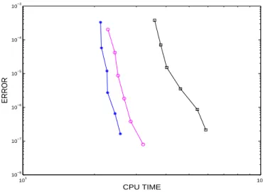
p X
l=0 τl
l!∂A
lu(t n).
(19)
232
We notice that ˜v0,n,tn(τ) is the same type of function which was considered with
233
Lawson methods. In case un wereu(tn), it corresponds to (15) with α=u(tn) and 234
therefore ˜v0,n,tn(k) is the same as (16) withτ=kandα=u(tn). If just∂u(tn) =∂un,
235
that solution would be the one given in Lemma 3.1 of [4] and, even in the case that
236
∂un 6=∂u(tn), ˜v0,n,tn(τ) would be understood in the sense described in Remark 2.3
237
of [4]. However, because of the assumed regularity off we want to remark here that
238
we do not need an initial boundary value problem similar to (15) to define the rest
239
of terms in (18). Nevertheless, we seek a differential equation which the functions in
240
(17) satisfy so that it is not necessary to calculateAlf(t
n+cik) (l= 0, . . . , p) on the 241
whole domain. For that, let us first consider the following lemma.
242
Lemma 6. Forj≥1andα∈X,
d
dτϕj(τ A0)α= (A0− j
τI)ϕj(τ A0)α+ 1
(j−1)!τα, τ >0,
where, for α∈X\D(A0), asD(A0)is dense in X,A0ϕj(τ A0)αis understood as the 243
corresponding limit of a sequence in D(A0). (This limit exists because, over D(A0),
244
A0ϕj(τ A0) = [ϕj−1(τ A0)−(j−1)!1 I]/τ, which is a bounded operator according to the
245
assumed hypotheses in the preliminaries.)
246
Proof. Assuming firstly thatα∈D(A0) and considering (2),
247
d dτ
1
τj Z τ
0
e(τ−θ)A0α θ
j−1
(j−1)!dθ
248
=− j
τj+1
Z τ
0
e(τ−θ)A0α θ
j−1
(j−1)!dθ+ 1 τj
τj−1 (j−1)!α+
1 τj
Z τ
0
A0e(τ−θ)A0α θ
j−1
(j−1)!dθ
249
= (A0−j
τI)ϕj(τ A0)α+ 1 (j−1)!τα.
250
The result on the whole spaceX comes from density.
251
From here, the next result follows:
252
problem:
254
vj0(τ) = (A−j
τ)vj(τ) + 1
(j−1)!τα, τ >0,
255
vj(0) =
1 j!α,
256
∂vj(τ) = p−1
X
l=0 τl
(l+j)!∂A
lα.
(20)
257
Proof. Notice that, using Lemma6,
258
vj0(τ) =
p−1
X
l=1 lτl−1 (l+j)!A
lα+pτp−1ϕ
p+j(τ A0)Apα 259
+τp[(A0− p+j
τ I)ϕp+j(τ A0) + 1
(p+j−1)!τI]A
pα 260
=
p−1
X
l=1 lτl−1 (l+j)!A
lα+ τ p−1
(p+j−1)!A
pα−jτp−1ϕ
p+j(τ A0)Apα+τpA0ϕp+j(τ A0)Apα. 261
On the other hand,
262
(A− j
τ)vj(τ) + 1 (j−1)!τα
263
=
p−1
X
l=0 τl
(l+j)!A
l+1α+τpAϕ
p+j(τ A0)Apα−j p−1
X
l=1 τl−1 (l+j)!A
lα−jτp−1ϕ
p+j(τ A0)Apα 264
=
p−1
X
m=1 m (m+j)!τ
m−1Amα+ τp−1
(p−1 +j)!A
pα−jτp−1ϕ
p+j(τ A0)Apα+τpAϕp+j(τ A0)Apα,
265
where the changem=l+1 has been used in the third line for the first sum. Therefore,
266
the lemma is proved taking also into account thatϕp+j(τ A0)Apα∈D(A0).
267
With Lawson methods [4], starting from a previous approximationUh,ntoPhu(tn) 268
and discretizing (19) in space led to a term like
269
Vh,n,0(k) =ekAh,0Uh,n+ p X
j=1
kjϕj(kAh,0)[AhQh∂Aj−1u(tn)−LhQh∂Aju(tn)] 270
+kp+1ϕp+1(kAh,0)AhQh∂Apu(tn),
(21)
271
which is the approximation which corresponds to the first term in (8).
272
For the rest of the terms in (8), we suggest to discretize (20) in space withα=
273
f(tn+cik). In such a way, the following system turns up: 274
Vh,j,n,i0 (τ) +LhQh∂vˆj,n,i0 (τ) =Ah,0Vh,j,n,i(τ) +AhQh∂ˆvj,n,i(τ)−
j
τ[Vh,j,n,i(τ) +LhQh∂vˆj,n,i(τ)]
275
+ 1
(j−1)!τ[Phf(tn+cik) +LhQh∂f(tn+cik)],
276
Vh,j,n,i(0) +LhQh∂ˆvj,n,i(0) =
1
j!Lhf(tn+cik),
where
278
ˆ
vj,n,i(τ) = p−1
X
l=0 τl (l+j)!A
lf(t
n+cik). 279
This can be rewritten as
280
Vh,j,n,i0 (τ) = (Ah,0− j
τI)Vh,j,n,i(τ) +AhQh∂vˆj,n,i(τ) + 1
(j−1)!τPhf(tn+cik)
281
+LhQh∂[
1
(j−1)!τf(tn+cik)− j
τvˆj,n,i(τ)−ˆv 0
j,n,i(τ)], 282
Vh,j,n,i(0) =
1
j!Phf(tn+cik). (22)
283
With the same arguments as in Lemma6,ϕj(τ Ah,0)Phf(tn+cik) is the solution of 284
Wh,j,n,i0 (τ) = (Ah,0− j
τI)Wh,j(τ) + 1
(j−1)!τPhf(tn+cik),
285
Wh,j,n,i(0) =
1
j!Phf(tn+cik).
286
Therefore, in order to solve (22), we are interested in finding
287
Zh,j,n,i(τ) =Vh,j,n,i(τ)−Wh,j,n,i(τ),
(23)
288
which is the solution of
289
Zh,j,n,i0 (τ) = (Ah,0− j
τI)Zh,j,n,i(τ) +AhQh∂vˆj,n,i(τ)
290
+LhQh∂[
1
(j−1)!τf(tn+cik)− j
τvˆj,n,i(τ)−vˆ 0
j,n,i(τ)], 291
Zh,j,n,i(0) = 0.
(24)
292
Now, using the first line of (20) for the boundary withα=f(tn+cik), 293
∂[ 1
(j−1)!τf(tn+cik)− j
τˆvj,n,i(τ)−vˆ 0
j,n,i(τ)] =−∂Avj,n,i(τ) 294
=− p−1
X
l=0 τl
(l+j)!∂A
l+1f(t
n+cik)−τp∂A0ϕp+j(τ A0)Apf(tn+cik), 295
the fact that
296
τpA0 1 τp+j
Z τ
0
e(τ−σ)A0 σ
p+j−1
(p+j−1)!A
pf(t
n+cik)dσ 297
=−1
τje
(τ−σ)A0 σ
p+j−1
(p+j−1)!|
σ=τ σ=0A
pf(t
n+cik) +
1 τj
Z τ
0
e(τ−σ)A0 σ
p+j−2
(p+j−2)!A
pf(t
n+cik)dσ 298
=− τ
p−1
(p+j−1)!A
pf(t
n+cik) +τp−1ϕp+j−1(τ A0)Apf(tn+cik), 299
and that the boundary of the second term vanishes, it follows that
300
∂[ 1
(j−1)!τf(tn+cik)− j
τvˆj,n,i(τ)−ˆv 0
j,n,i(τ)] =− p−2
X
l=0 τl (l+j)!∂A
l+1f(t
Using this in (24),
302
Zh,j,n,i(τ) 303
=
Z τ
0
eRθτ(Ah,0− j σI)dσ
p−2
X
l=0 θl (l+j)!
AhQh∂Alf(tn+cik)−LhQh∂Al+1f(tn+cik) 304
+ θ
p−1
(p−1 +j)!AhQh∂A
p−1f(t
n+cik)
dθ
305
=
p−2
X
l=0
Z τ
0
eAh,0(τ−θ) θ
j+l
τj(l+j)![AhQh∂A lf(t
n+cik)−LhQh∂Al+1f(tn+cik)]dθ 306
+
Z τ
0
eAh,0(τ−θ) θ
p−1+j
τj(p−1 +j)!AhQh∂A p−1f(t
n+cik)dθ 307
=
p−2
X
l=0
τl+1ϕj+l+1(τ Ah,0)[AhQh∂Alf(tn+cik)−LhQh∂Al+1f(tn+cik)] 308
+τpϕp+j(τ Ah,0)AhQh∂Ap−1f(tn+cik).
(25)
309
Therefore, using (23),
310
Vh,j,n,i(k) =ϕj(kAh,0)Phf(tn+cik) 311
+
p−2
X
l=0
kl+1ϕj+l+1(kAh,0)[AhQh∂Alf(tn+cik)−LhQh∂Al+1f(tn+cik)], 312
+kpϕp+j(kAh,0)AhQh∂Ap−1f(tn+cik),
(26)
313
and the overall exponential quadrature rule would be given by
314
Uh,0=Phu0, 315
Uh,n+1=Vh,n,0(k) +k
s X
i,j=1
ai,jVh,j,n,i(k),
(27)
316
withVh,n,0(k) in (21) andVh,j,n,i(k) in (26). 317
4.1. Time semidiscretization error. Let us first study just the error after
318
time discretization. The local truncation error is well-known to be given by ρn = 319
u(tn+1)−u¯n+1, where ¯un+1 is given by expression (18) substitutingun byu(tn). 320
Let us first consider the following general result, which will allow to conclude
321
more particular results depending on the choice of the values{ci}s i=1.
322
Lemma 8. Under the assumptions of regularity (4), the local truncation error
satisfies
ρn= p X
m=1 km
m−1 X
r=0 1 m!−
1 r!
s X
l=1
1 (m−r−1 +l)!
s X
i=1
criailAm−r−1f(r)(tn)
+O(kp+1).
Proof. Notice that ¯un+1 can be written as
324
¯
un+1=u(tn) + p X
j=1 kj
1
j!A
ju(t n) +
s X
i,l=1 ai,l
1 (j−1 +l)!A
j−1f(t
n+cik)
+O(kp+1)
325
=u(tn) + p X j=1 kj 1 j!A
ju(t n) +
s X
i,l=1 ai,l
1 (j−1 +l)!
p−j X
r=0 crikr
r! A
j−1f(r)(t
n)
+O(kp+1)
326
=u(tn) + p X
m=1 km
1
m!A
mu(t n) +
s X i,l=1 ai,l m−1 X r=0 cr i
(m−r−1 +l)!r!A
m−r−1f(r)(t
n)
+O(kp+1),
327
where the Taylor expansion of f(tn +cik) has been used as well as changes of 328
subindexes.
329
As, according to (1),
330
u(tn+1) =u(tn) + p X
m=1 km m!u
(m)(t
n) 331
=u(tn) + p X
m=1 km m![A
mu(t n) +
m−1
X
r=0
Am−r−1f(r)(tn)] +O(kp+1), 332
the result follows.
333
Theorem 9. If p=sin (4) and (18), for any nodes {ci}si=1,ρn =O(ks+1). 334
Proof. It suffices to take into account that any polynomial of degree≤s−1 coin-cides with its interpolant on the nodes{ci}si=1. Therefore, forr≤s−1,
Ps i=1c
r ili(θ) =
θr. Using (7), this implies that
s X
i=1
cri ai,l (l−1)! =
0 if l6=r+ 1 1 if l=r+ 1,
or equivalently, forr≤s−1,
s X
i=1
criai,r+1=r!,
s X
i=1
criai,l= 0, wheneverl6=r+ 1.
Substituting this in the expression for ρn in Lemma8 with p= s, all the terms in 335
brackets vanish and the result follows.
336
Theorem 10. If p=s+ 1in (4) and (18) and the nodes {ci}si=1 are such that
337
the interpolatory quadrature rule which is based on them is exact for polynomials of
338
degree≤s,ρn=O(ks+2). 339
Proof. With the same argument as in the previous lemma, all the terms in brack-ets in the expression of ρn in Lemma 8 vanish form≤s. Then, form=s+ 1, the
term in parenthesis vanishes for the same reason when r≤s−1. It just suffices to see what happens whenm=s+ 1 and r=s. But, as the quadrature rule which is based on{ci}s
i=1 is assumed to be exact for the polynomialθs,
1 s+ 1 =
Z 1
0
θsdθ=
Z 1
0
s X
i=1
csili(θ)dθ= s X
i=1 csi
s X
l=1 ai,l
l! .
From this, the result also directly follows.
We now state the following much more general result:
341
Theorem 11. Whenever the nodes{ci}si=1are such that the interpolatory
quadra-342
ture rule which is based on them is exact for polynomials of degree≤p−1, considering
343
that value of pin (4) and (18), ρn =O(kp+1). 344
Proof. It suffices to notice that, for 0 ≤ r ≤ m−1, with m ≤ p, due to the
345
hypothesis,
346
Z 1
0
Z u1
0 . . .
Z um−r−1
0
θrdθdum−r−1. . . du1
347
=
Z 1
0
Z u1
0 . . .
Z um−r−1
0
s X
i=1
crili(θ)dθdum−r−1. . . du1.
348
Now, the left-hand side term above can inductively be proved to be
1 r+ 1
1 r+ 2. . .
1 m,
and the right-hand side can be written as
349
Z 1
0
Z u1
0 . . .
Z um−r−1
0
s X
i=1 cri
s X
l=1 ai,l
θl−1
(l−1)!dθdum−r−1. . . du1
350
=
s X
l=1
s X
i=1 criai,l
Z 1
0
Z u1
0 . . .
Z um−r−1
0
θl−1
(l−1)!dθdum−r−1. . . du1
351
=
s X
l=1
s X
i=1 criai,l
1
(l−1 +m−r)!.
352
Then, using Lemma8, the result directly follows.
353
From this, the following interesting results are achieved:
354
Corollary 12. (i) For thesnodes corresponding to a Gaussian
quadra-355
ture rule, considering p= 2s in (4) and (18),ρn=O(k2s+1). 356
(ii) For thesnodes corresponding to a Gaussian-Lobatto quadrature rule,
con-357
sidering p= 2s−2 in (4) and (18),ρn =O(k2s−1). 358
Remark 13. Due to the fact that the last node of one step is the first of the
359
following, the nodes corresponding to the Gaussian-Lobatto quadrature rule have the
360
advantage that justs(s−1)(instead ofs2) terms of the formV
h,n,j,imust be calculated 361
in (27).
362
4.2. Full discretization error. Let us also consider the error which arises when
363
discretizing (15) and (20) in space.
364
4.2.1. Local error. To define the local error after full discretization, we consider ¯
Uh,n+1= ¯Vh,n,0(k) +k
s X
i,j=1
ai,jV¯h,n,j,i(k),
where
365
(i) ¯Vh,n,0(τ) is the solution of
366
¯
Vh,n,0 0(τ) +LhQh∂vˆn,0 0(τ) =Ah,0V¯h,n,0(τ) +AhQh∂vˆn,0(τ),
367
¯
Vh,n,0(0) =Rhu(tn), 368
with ˆvn,0(τ) =
Pp l=0
τl
l!A
(ii) ¯Vh,n,j,i(τ) is the solution of (22) substitutingPhf(tn+cik) byRhf(tn+cik). 370
More precisely,
371
¯
Vh,j,n,i0 (τ) = (Ah,0− j
τI) ¯Vh,j,n,i(τ) +AhQh∂vˆj,n,i(τ)
372
+ 1
(j−1)!τRhf(tn+cik)
373
+LhQh∂[
1
(j−1)!τf(tn+cik)− j
τˆvj,n,i(τ)−vˆ 0
j,n,i(τ)], 374
¯
Vh,j,n,i(0) =
1
j!Rhf(tn+cik). (28)
375
Then, we defineρh,n=Rhu(tn+1)−U¯h,n+1 and the following is satisfied.
376
Theorem 14. Let us assume that, apart from hypotheses of Section 2,u and f
377
in (1) satisfy
378
Aju∈C([0, T], Z), j= 0, . . . , p+ 1, Ajf ∈C([0, T], Z), j= 0, . . . , p. (29)
379
Then, ρh,n =O(kεh+kρnk), where the constant in Landau notation is independent 380
of kandhand the bounds in Section 4.1hold forρn. 381
Proof. Because of definition,
382
ρh,n= (Rhu(tn+1)−Rhu¯n+1) + (Rhu¯n+1−U¯h,n+1)
383
=Rhρn+ (Rhu¯n+1−U¯h,n+1), (30)
384
where ¯un and ρn are those defined in Section 4.1. The fact that (29) is satisfied 385
implies that ¯un+1 belongs toZ and thereforeρn ∈Z. Moreover, kρnkZ =O(kρnk) 386
and, using the same proof as that of Theorem 11 in [4],
387
Rhρn=O(kρnk).
(31)
388
On the other hand,
389
Rhu¯n+1−U¯h,n+1=Rh¯v0,n−V¯h,n,0(k) +k
s X
i,j=1
ai,j[Rhvj,n,i(k)−V¯h,j,n,i(k)],
(32)
390
where ¯v0,n corresponds to (16) withα=u(tn) andvj,n,i(τ) corresponds to (17) with 391
α=f(tn+cik). In the same way as in the proof of Theorem 4.4 in [4], 392
Rhv0¯,n−V¯h,n,0(k) =O(kεh).
(33)
393
Moreover, using Lemma7,
394
Rhvj,n,i0 (τ) =RhAvj,n,i(τ)−
j
τRhvj,n,i(τ) + 1
(j−1)!τRhf(tn+cik)
395
=PhAvj,n,i(τ) + (Rh−Ph)Avj,n,i(τ)−
j
τRhvj,n,i(τ) + 1
(j−1)!τRhf(tn+cik)
396
=Ah,0Rhvj,n,i(τ) +AhQh∂vˆj,n,i(τ)−LhQh∂Avj,n,i(τ) 397
+(Rh−Ph)Avj,n,i(τ)−
j
τRhvj,n,i(τ) + 1
(j−1)!τRhf(tn+cik),
and making the difference with (28), it follows that
399
Rhvj,n,i0 (τ)−V¯h,n,j,i0 (τ) = (Ah,0− j
τI)(Rhvj,n,i(τ)−Vh,n,j,i(τ)) + (Rh−Ph)Avj,n,i,
400
where we have used that
∂[Avj,n,i(τ) +
1
(j−1)!τf(tn+cik)− j
τ∂ˆvj,n,i(τ)−∂vˆ 0
j,n,i(τ)] = 0
because of Lemma7. Now, due to the same lemma and (28),Rhvj,n,i(0)−V¯h,n,j,i(0) = 401
0, and therefore
402
Rhvj,n,i(k)−V¯h,n,j,i(k) = Z k
0
e(k−τ)Ah,0τ
j
kj(Rh−Ph)Avj,n,i(τ)dτ 403
=kϕj+1(kAh,0)O(εh) =O(kεh).
(34)
404
Here we have used that Avj,n,i∈ Z because of (29) and Lemma 3.3 in [4]. Finally, 405
gathering (30)–(34), the result follows.
406
4.2.2. Global error. We now study the global error, which we define aseh,n= 407
Phu(tn)−Uh,n. 408
Theorem 15. Under the same assumptions of Theorem 14,
409
eh,n=O(
1
k0≤maxl≤n−1kρlk+εh),
410
where the constant in Landau notation is independent of k and hand the bounds in
411
Section4.1 hold forρl. 412
Proof. As in the proof of Theorem 4.5 in [4],
413
eh,n+1= (Phu(tn+1)−Rhu(tn+1)) +Rhu(tn+1)−Uh,n+1
414
=O(εh) +Rhu(tn+1)−Uh,n+1.
(35)
415
The difference is that now, using (27),
416
Rhu(tn+1)−Uh,n+1=ρh,n+Uh,n+1−Uh,n+1
417
=ρh,n+ ¯Vh,n,0(k)−Vh,n,0(k) +k
s X
i,j=1
aij( ¯Vh,j,n,i(k)−Vh,j,n,i(k)). 418
As in [4],
419
¯
Vh,n,0−Vh,n,0=ekAh,0(Rhu(tn)−Uh,n). 420
As for ¯Vh,j,n,i(k)−Vh,j,n,i(k), making the difference between (28) and (22), 421
¯
Vh,j,n,i0 (τ)−Vh,j,n,i0 (τ) = (Ah,0− j
τ)( ¯Vh,j,n,i(τ)−Vh,j,n,i(τ)) + 1
(j−1)!τ(Rh−Ph)f(tn+cik),
422
¯
Vh,j,n,i(0)−Vh,j,n,i(0) =
1
j!(Rh−Ph)f(tn+cik).
423
Considering then an analogue of Lemma 6 substituting A0 byAh,0 and taking into
424
account thatϕj(0) = 1/j! (3), 425
¯
Therefore,
427
Rhu(tn+1)−Uh,n+1=ekAh,0(Rhu(tn)−Uh,n) +ρh,n+O(kεh). 428
This implies that
Rhu(tn+1)−Uh,n+1=etn+1Ah,0(Rhu(0)−Uh,0) +O( 1
k0≤maxl≤nkρh,lk+εh),
which, together with the first line of (27), (10), (35) and Theorem 14, implies the
429
result.
430
5. Numerical experiments. In this section we will show some numerical
exper-431
iments which corroborate the previous results. For that, we have considered parabolic
432
problems with homogeneous and non-homogeneous Dirichlet boundary conditions for
433
which X = L2(Ω) for a certain spatial domain Ω and g ∈ H1
2(∂Ω). The fact that
434
these problems can be well fitted under the theory of abstract IBVPs is well
justi-435
fied in [4, 13]. Moreover, other types of boundary conditions can also be considered
436
although we restrict here to Dirichlet boundary conditions just for the sake of brevity.
437
As for the space discretization, we have considered here both the standard
sym-438
metric 2nd-order finite differences and collocation spectral methods in 1 dimension.
439
For the former, it was already well justified in [4] that the hypotheses which are
440
required on the space discretization are satisfied, at least for the discrete L2-norm,
441
Z=H4(Ω) andε
h=O(h2). Besides, a discrete maximum principle (hypothesis (HS)) 442
is well-known to apply [14]. With the collocation spectral methods, those hypotheses
443
are also valid with the discrete L2-norm associated to the corresponding
Gaussian-444
Lobatto quadrature rule (k · kh,GL), Z = Hm(Ω) and εh = O(J2−m) [2, 6], where 445
J+ 1 is the number of collocation nodes, which is clearly inversely proportional to the
446
diameter space gridh. In such a way, the more regular the functions are, the quicker
447
the numerical solution of the elliptic problems converges to the exact solution.
448
Besides, although in the collocation case the matrix which representsAh,0 is not
449
symmetric any more, Remarks3and5still apply. Notice that, for every matrixBof
450
dimension (J −1)×(J−1),
451
kBkh,GL=kDJBDJ−1kh
(36)
452
where DJ denotes the diagonal matrix which contains the square root of the
co-efficients of the quadrature rule corresponding to the interior Gauss-Lobatto nodes
{xj}J−1
j=1. (We will denote them by {αj}
J−1
j=1.) Because of this, when DJBDJ−1 is
symmetric, kBkh,GL = ρ(B). The fact that DJAh,0DJ−1 is symmetric comes from
the following: Notice that (Ah)i,j =L00j(xi) where {Lj(x)}are the Lagrange
polyno-mials associated to the interior Gauss-Lobatto nodes and those at the boundary. As
{Lj(x)}jJ=1−1vanish at the boundary, integrating by parts, for everyi, j∈ {1, . . . , J−1},
Z
L00j(x)Li(x)dx=− Z
L0j(x)L0i(x)dx.
As the integrand in the left-hand side is a polynomial of degree 2J −2, the corre-sponding Gaussian-Lobatto quadrature rule integrates it exactly. Therefore,
αiL00j(xi) =− Z
where, for the last equality, the role ofiandj has been interchanged. From this, and using (36) again,
kkAh,0
n−1
X
r=1
erkAh,0k
h,GL=kkDJAh,0D−1J e
k(1−θ)DJAh,0DJ−1kh.
AsDJAh,0DJ−1 is symmetric, the matrix insidek · kh is also symmetric and therefore
kkAh,0
n−1
X
r=1
erkAh,0kh,GL=ρ(kD
JAh,0D−1J n−1
X
r=1
erkDJAh,0D−J1) =ρ(kAh,0
n−1
X
r=1
erkAh,0).
Secondly, the eigenvalues ofAh,0 are negative. This is due to the following: For every polynomial which vanishes at the boundary such thatp(x)6≡0,
Z
p00(x)p(x)dx=− Z
[p0(x)]2dx <0.
Considering p(x) =PJi=1−1βiLi(x) and using the Gauss-Lobatto quadrature rule and
the definition of Lagrange polynomials,
J−1
X
k=1 αk(
J−1
X
i=1
βiL00i(xk))( J−1
X
j=1
βjLj(xk)) = J−1
X
i,k=1
αkβiβkL00i(xk)<0.
This can be rewritten as ~βTD2
JAh,0β <~ 0 for every vector β~ 6=~0, or equivalently,
453
(DJβ~)TDJAh,0D−1J (DJβ~)<0, which implies thatDJAh,0D−1J has negative eigenval-454
ues and so hasAh,0.
455
For both types of discretizations which have been considered here, LhQh∂ ≡0 456
and therefore formulas (21) and (26) simplify a little bit. However, other possible
dis-457
cretizations (as those considered in [4]) are also possible, for which that simplification
458
cannot be made.
459
In all cases, we have considered the one-dimensional problem
460
ut(x, t) =uxx(x, t) +f(x, t), 0≤t≤1, 0≤x≤1, 461
u(x,0) =u0(x),
462
u(0, t) =g0(t), u(1, t) =g1(t), (37)
463
with the corresponding functionsf, u0, g0 and g1 which make thatu(x, t) =x(1−
464
x)e−toru(x, t) =ex−tare solutions of the problem. These functions satisfy regularity 465
hypotheses (4) and (29) for any natural numberp.
466
5.1. Trapezoidal rule. We begin by considering the trapezoidal rule in time
467
and the second-order finite differences in space. We have consideredh= 10−3so that
468
the error in space is negligible. The trapezoidal rule corresponds tos= 2 but is just
469
exact for polynomials of degree≤1. Therefore, one of the hypothesis of Theorem2is
470
not satisfied and we can just apply Theorem1when discretizating firstly in space and
471
then in time with the solution which satisfiesg0(t) =g1(t) = 0. That theorem states
472
that, with respect to the time stepsizek, the local and global error should show orders
473
3 and 2 respectively and we can check that really happens in Table 1. For the same
474
problem, but applying the technique which is suggested in this paper (27) withp= 2,
475
Theorems9,14and15state that also the local and global error should show orders 3
Classical approach Suggested approach
k Loc. err. ord. Glob. err. ord. Loc. err. ord. Glob. err. ord.
1/10 8.0170e-5 5.5395e-5 1.5334e-4 9.8091e-5
1/20 1.2961e-5 2.6 1.3953e-5 2.0 1.9139e-5 3.0 1.8575e-5 2.4 1/40 1.8644e-6 2.8 3.4952e-6 2.0 2.3902e-6 3.0 4.0262e-6 2.2 1/80 2.5316e-7 2.9 8.7426e-7 2.0 2.9862e-7 3.0 9.3773e-7 2.1 1/160 3.3354e-8 2.9 2.1860e-7 2.0 3.7318e-8 3.0 2.2635e-7 2.0 1/320 4.3171e-9 3.0 5.4651e-8 2.0 4.6641e-9 3.0 5.5610e-8 2.0
Table 1
Trapezoidal rule,h= 10−3,u(x, t) =x(1−x)e−t
Classical approach Suggested approach
k Loc. err. ord. Glob. err. ord. Loc. err. ord. Glob. err. ord.
1/10 7.4531e-4 4.8108e-4 2.0144e-4 1.3742e-4
1/20 1.5446e-4 2.3 1.2476e-4 2.0 2.8775e-5 2.8 3.0165e-5 2.2 1/40 3.3863e-5 2.2 3.2074e-5 2.0 3.9084e-6 2.9 7.0453e-6 2.1 1/80 7.3906e-6 2.2 8.1809e-6 2.0 5.1475e-7 2.9 1.6979e-6 2.0 1/160 1.5848e-6 2.2 2.0770e-6 2.0 6.6122e-8 3.0 4.1324e-7 2.0 1/320 3.3666e-7 2.2 5.2777e-7 2.0 8.1531e-9 3.0 9.8459e-8 2.1
Table 2
Trapezoidal rule,h= 10−3,u(x, t) =ex−t
and 2 respectively and that is what we can in fact observe in the same table. We can
477
see that, although the local order is a bit more clear with the suggested technique, the
478
size of the errors is slightly bigger with the suggested approach. Therefore, it seems
479
that, in this particular problem, the error constants are bigger with the suggested
480
technique and it is not worth the additional cost of calculating terms which contain
481
ϕ3(kAh,0) andϕ4(kAh,0).
482
The comparison is more advantageous for the suggested technique when the
solu-483
tion is such that it does not vanish at the boundary. Then, Theorem4and Remark5 484
state that the local and global error should show order 2 with the classical approach
485
and that can be checked in Table 2. However, with the suggested strategy, as with
486
the vanishing boundary conditions case, the theorems in this paper prove local order
487
3 and global order 2, which can again be checked in the same table. The fact that we
488
manage to increase the order in the local error makes that the global errors, although
489
always of order 2, are smaller with the suggested technique than with the classical
ap-490
proach. Nevertheless, the comparison between both techniques will be more beneficial
491
for the technique which is suggested in the paper when the classical (non-exponential)
492
order of the quadrature rule increases.
493
5.2. Simpson rule. In this subsection we consider Simpson rule in time and
494
a collocation spectral method in space with 40 nodes so that the error in space is
495
negligible. As Simpson rule corresponds to s = 3 and the interpolatory quadrature
496
rule which is based in those 3 nodes is exact for polynomials of degree ≤3, we can
497
take p= 4 in Theorem10 and achieve orders 5 and 4 for the local and global error
498
respectively with the technique suggested here. However, with the classical approach,
499
at least in the common case thatg(t)6≡0, Theorem4and Remark5give just order 3
500
for the local and global error. These results can be checked in Table3. Moreover, the
Classical approach Suggested approach
k Loc. err. ord. Glob. err. ord. Loc. err. ord. Glob. err. ord.
1/2 8.0718e-4 4.9507e-4 2.7496e-4 1.6821e-4
1/4 8.3265e-5 3.3 4.2862e-5 3.5 8.5778e-6 5.0 4.4156e-6 5.2 1/8 8.6214e-6 3.3 4.0561e-6 3.4 2.6785e-7 5.0 1.5345e-7 4.8 1/16 1.0500e-6 3.0 4.4103e-7 3.2 8.3681e-9 5.0 6.7803e-9 4.5 1/32 1.1622e-7 3.2 4.6864e-8 3.2 2.6148e-10 5.0 3.5342e-10 4.3 1/64 1.2378e-8 3.2 4.9423e-9 3.2 8.1711e-12 5.0 2.0189e-11 4.1
Table 3
Simpson’s rule,J= 61,u(x, t) =ex−t
Classical approach Suggested approach
k Loc. err. ord. Glob. err. ord. Loc. err. ord. Glob. err. ord.
1/4 8.2639e-3 4.3743e-3 4.9483e-3 2.5685e-3
1/8 1.8874e-3 2.1 1.1548e-3 1.9 6.4427e-4 2.9 3.7820e-4 2.8 1/16 3.6716e-4 2.4 2.9791e-4 2.0 8.2199e-5 3.0 6.9202e-5 2.4 1/32 7.6916e-5 2.2 7.6389e-5 2.0 1.0381e-5 3.0 1.4677e-5 2.2 1/64 1.6803e-5 2.2 1.9445e-5 2.0 1.3043e-6 3.0 3.3796e-6 2.1 1/128 3.6111e-6 2.2 4.9232e-6 2.0 1.6345e-7 3.0 8.1115e-7 2.1
Table 4
Midpoint rule,J= 61,u(x, t) =x(1−x)e−t
size of the global error, even for the bigger timestepsizes is smaller with the suggested
502
technique.
503
We also want to remark here that the trapezoidal and Simpson rules correspond
504
to Gauss-Lobatto quadrature rules withs = 2 ands = 3 respectively and therefore
505
Corollary12(ii) and Remark13apply.
506
5.3. Gaussian rules. In order to achieve the highest accuracy given a certain
507
number of nodes, we consider in this subsection Gaussian quadrature rules. More
508
precisely, those corresponding tos= 1,2,3,4. As space discretization, we have
con-509
sidered again the same spectral collocation method of the previous subsection.
Fol-510
lowing Corollary12(i) and Theorem14, even for non-vanishing boundary conditions,
511
takingp= 2sin (21) and (26) the local error in time should show order 2s+ 1 and the
512
global error, using Theorem 15, order 2s. This should be compared with the order
513
s+ 1 which is proved for the classical approach when g(t)≡0 in Theorem2 and the
514
ordersfor the local and global error wheng(t)6≡0, which comes from Theorem4and
515
Remark5. In Tables4 and5we see the results which correspond tos= 1 ands= 2
516
respectively for the vanishing boundary conditions case. Although fors= 1 there is
517
not an improvement on the global order for the suggested technique, the errors are a
518
bit smaller. Of course the benefits are more evident withs= 2. For the non-vanishing
519
boundary conditions case, Tables 6,7,8 and 9 show the results which correspond to
520
s= 1,2,3 and 4 respectively. When avoiding order reduction, the results are much
521
better than with the classical approach. Not only the order is bigger but also the size
522
of the errors is smaller from the very beginning. We notice that the global order is
523
even a bit better than expected for the first values ofk.
524
Finally, although it is not an aim of this paper, in order to compare roughly the
Classical approach Suggested approach
k Loc. err. ord. Glob. err. ord. Loc. err. ord. Glob. err. ord.
1/2 8.9292e-4 5.4788e-4 8.2591e-5 5.0573e-5
1/4 8.6746e-5 3.4 4.5296e-5 3.6 2.8465e-6 4.9 1.4782e-6 5.1 1/8 8.1186e-6 3.4 3.9933e-6 3.5 9.3457e-8 4.9 5.4928e-8 4.7 1/16 1.0237e-6 3.0 4.3449e-7 3.2 2.9938e-9 5.0 2.5254e-9 4.4 1/32 1.1415e-7 3.2 4.6048e-8 3.2 9.4726e-11 5.0 1.3424e-10 4.2 1/64 1.2112e-8 3.2 4.8418e-9 3.2 2.9786e-12 5.0 7.7190e-12 4.1
Table 5
Gaussian rule withs= 2,J= 61,u(x, t) =x(1−x)e−t
Classical approach Suggested approach
k Loc. err. ord. Glob. err. ord. Loc. err. ord. Glob. err. ord.
1/8 6.6985e-2 2.8814e-2 1.5650e-3 8.6254e-4
1/16 3.0444e-2 1.1 1.2167e-2 1.2 1.8673e-4 3.1 1.4048e-4 2.6 1/32 1.3218e-2 1.2 5.1128e-3 1.2 2.2356e-5 3.1 2.7661e-5 2.3 1/64 5.6269e-3 1.2 2.1472e-3 1.2 2.6947e-6 3.1 6.1319e-6 2.2 1/128 2.3791e-3 1.2 9.0138e-4 1.2 3.2718e-7 3.0 1.4450e-6 2.1 1/256 1.0015e-3 1.2 3.7813e-4 1.2 3.9993e-8 3.0 3.5085e-7 2.0
Table 6
Midpoint rule,J= 61,u(x, t) =ex−t
results in terms of computational cost, let us concentrate on Gaussian quadrature
526
rules of the same order 2swhen integrating a non-vanishing boundary value problem.
527
When considering 2snodes with the classical approach, 2sevaluations of the source
528
termf must be made at each step and the 2soperators{ϕj(kAh,0)}2j=1s are needed,
529
which will be multiplied by vectors with all its components varying in principle at
530
each step. However, with the suggested technique ands nodes, justsevaluations of
531
the source termf must be made although 3s operators {ϕj(kAh,0)}3j=1s are needed.
532
Nevertheless, from these 3s, just the firsts of them are multiplied by vectors which
533
change independently in all their components at each step. The other 2s are
mul-534
tiplied by vectors which just contain information on the boundary. Therefore, with
535
finite differences many components vanish and, with Gauss-Lobatto spectral methods,
536
those vectors are just a time-dependent linear combination of two vectors which do not
537
change with time. With Gauss-Lobatto methods, asAh,0 is not sparse but its size is
538
moderate, we have calculated once and for all at the very beginningekAh,0,ϕ
j(kAh,0),
539
j= 1, . . . , sand the two necessary vectors derived fromϕj(kAh,0),j=s+ 1, . . . ,3s.
540
Then, in (27) the terms containing the former at each step requireO(J2) operations
541
while the terms containing the latter just requireO(J) operations. With finite
differ-542
ences, as the matrixAh,0is sparse and usually bigger, we have applied general Krylov
543
subroutines [11] to calculate all the required terms at each step.
544
We offer a particular comparison for order 2 with Gauss-Lobatto spectral space
545
discretization on the one hand and 2nd-order finite differences on the other, and
546
considering the implementation described above in each case. In Figure1we can see
547
that, for the former, the suggested technique is more than twice cheaper than the
548
classical one and, with the latter in Figure2, the comparison is not so advantageous
549
for the suggested technique but it is still cheaper than the classical approach. We also
Classical approach Suggested approach
k Loc. err. ord. Glob. err. ord. Loc. err. ord. Glob. err. ord.
1/2 1.9328e-2 1.1743e-2 7.9408e-4 4.8503e-4
1/4 4.8715e-3 2.0 2.3068e-3 2.3 2.2565e-5 5.1 1.1356e-5 5.4 1/8 1.1460e-3 2.1 4.7811e-4 2.3 6.3799e-7 5.1 3.3399e-7 5.1 1/16 2.5199e-4 2.2 9.8750e-5 2.3 1.8167e-8 5.1 1.2423ee-8 4.7 1/32 5.4061e-5 2.2 2.0543e-5 2.3 5.2222e-10 5.1 5.7608e-10 4.4 1/64 1.1476e-5 2.2 4.2930e-6 2.3 1.4918e-11 5.1 2.9580e-11 4.3
Table 7
Gaussian rule withs= 2,J= 61,u(x, t) =ex−t
Classical approach Suggested approach
k Loc. err. ord. Glob. err. ord. Loc. err. ord. Glob. err. ord.
1/2 8.4732e-4 5.1405e-4 3.0107e-6 1.8363e-6
1/4 1.0734e-4 3.0 5.0710e-5 3.3 2.0423e-8 7.2 1.0082e-8 7.5 1/8 1.2260 e-5 3.1 5.1107e-6 3.3 1.3840e-10 7.2 6.6752e-11 7.2 1/16 1.3379e-6 3.2 5.2398e-7 3.3 9.4087e-13 7.2 5.3198e-13 7.0 1/32 1.4335e-7 3.2 5.4413e-8 3.3 6.4275e-15 7.2 5.3534e-15 6.6 1/64 1.5182e-8 3.2 5.6735e-9 3.3 4.4259e-17 7.2 6.6517e-17 6.3
Table 8
Gaussian rule withs= 3,J= 61,u(x, t) =ex−t
remark that, in any case, the more expensive the source functionf is to evaluate, the
551
more advantageous the suggested technique withsnodes will be against the classical
552
approach with 2snodes.
553
Moreover, in the same figures, we also compare with the Lawson midpoint rule
554
avoiding order reduction according to [4], which is described in this case by
555
Uh,n+1=Vh,n,0(k) +k
ek2Ah,0P
hf(tn+
k 2) +
k 2ϕ1(
k
2Ah,0)AhQh∂f(tn+ k 2)
556
+1 4k
2ϕ 2(
k
2Ah,0)AhQh∂Af(tn+ k 2)
,
557
withVh,n,0 that in (21) withp= 2, i.e.,
558
Vh,n,0=ekAh,0Uh,n+kϕ1(kAh,0)AhQh∂u(tn) +k2ϕ2(kAh,0)AhQh∂Au(tn) 559
+k3ϕ3(kAh,0)AhQh∂A2u(tn). 560
If we compare with the exponential midpoint rule which is suggested in this paper,
561
which is given by
562
Uh,n+1=Vh,n,0(k) +k
ϕ1(kAh,0)Phf(tn+
k
2) +kϕ2(kAh,0)AhQh∂f(tn+ k 2)
563
+k2ϕ3(kAh,0)AhQh∂Af(tn+
k 2)
,
564
we can see that now there are no terms inek2Ah,0,ϕ1(k
2Ah,0),ϕ2(
k
2Ah,0) and moreover,
565
we can group together the terms inϕ1(kAh,0),ϕ2(kAh,0) andϕ3(kAh,0).
Classical approach Suggested approach
k Loc. err. ord. Glob. err. ord. Loc. err. ord. Glob. err. ord.
1/2 2.7746e-5 1.6829e-5 8.1253e-9 4.9495e-9
1/4 1.7137e-6 4.0 8.0951e-7 4.4 1.3502e-11 9.2 6.5604e-12 9.6 1/8 9.6826e-8 4.1 4.0363e-8 4.3 2.2443e-14 9.2 1.0107e-14 9.3 1/16 5.2833e-9 4.2 2.0690e-9 4.3 3.7267e-17 9.2 1.7380e-17 9.2 1/32 2.8240e-10 4.2 1.0719e-10 4.3 6.2266e-20 9.2 3.5644e-20 8.9
Table 9
Gaussian rule withs= 4,J= 61,u(x, t) =ex−t
When using the implementation which is described above for Gauss-Lobatto
spec-567
tral space discretization, those matrices are stored at the very beginning and the
568
advantage of the rule suggested here above Lawson one is not so big. Notice that,
569
with Lawson rule, 2 expensive applications of matrices over vectors are performed
570
(those corresponding to ekAh,0 and ek2Ah,0) while the other 5 ones corresponding to
571
ϕ1(kAh,0),ϕ2(kAh,0),ϕ3(kAh,0),ϕ1(k2Ah,0) andϕ2(k2Ah,0) are much cheaper because
572
they just act over the boundaries. Meanwhile, with the rule suggested here, again 2
573
of them are expensive (those corresponding to ekAh,0 and ϕ
1(kAh,0)) and there are
574
just other 2 (corresponding toϕ2(kAh,0) andϕ3(kAh,0)), which are cheap. Because of
575
this, the rule which is studied in this paper outperforms Lawson one but the difference
576
is not so big. (Look at Figure1.)
577
However, for more general problems in which the calculation or the storage of the
578
big matrices is not possible, the advantage of the rule studied here above Lawson is
579
much more pronounced, as it corresponds to calculating additionally through Krylov
580
methods the terms in ek2Ah,0, ϕ1(k
2Ah,0), ϕ2(
k
2Ah,0), which require approximately
581
the same cost as those inekAh,0,ϕ1(kA
h,0),ϕ2(kAh,0) andϕ3(kAh,0) and which are
582
needed with both methods [11]. That difference is clearly observed in Figure2.
583
Besides, although not explicitly done here for the sake of brevity, with the same
584
argument it can be deduced that the biggersis, the bigger the advantage of the rules
585
suggested here above Lawson ones.
586
REFERENCES 587
[1] I. Alonso–Mallo,Rational methods with optimal order of convergence for partial differential
588
equations, Appl. Num. Math.35(2000), 265–292. 589
[2] I. Alonso–Mallo, B. Cano and J. C. Jorge, Spectral-Fractional Step Runge-Kutta
Dis-590
cretizations for Initial Boundary Value Problems with Time-Dependent Boundary
Condi-591
tions, Math. Comput.73(2004), 1801–1825. 592
[3] I. Alonso–Mallo, B. Cano and N. Reguera, Analysis of order reduction when integrating
593
linear initial boundary value problems with Lawson methods, Appl. Numer. Math., 118 (2017) 594
64–74. 595
[4] I. Alonso–Mallo, B. Cano and N. Reguera,Avoiding order reduction when integrating linear
596
initial boundary value problems with Lawson methods, IMA J. Num. Anal., 37 (2017), 2091– 597
2119. 598
[5] I. Alonso–Mallo, B. Cano and N. Reguera, Avoiding order reduction when
inte-599
grating reaction-diffusion boundary value problems with exponential splitting methods, 600
arXiv:1705.01857. 601
[6] C. Bernardy and Y. Maday,Approximations spectrales de problemes aux limites elliptiques,
602
Springer-Verlag France, Paris, 1992. 603
[7] T. G¨ockler and V. Grimm,Convergence analysis of an extended Krylov subspace method for
604
the approximation of operator functions in exponential integrators, SIAM J. Numer. Anal. 605
10−4
10−3
10−2
10−1
10−7
10−6
10−5
10−4
10−3
CPU TIME
ERROR
Fig. 1. Error against CPU time when integrating problem (37) with exact solutionu(x, t) =
ex−t, using Gauss-Lobatto spectral method in space and, in time, the classical approach of Gaussian rule withs= 2(pink circles), the suggested technique for midpoint rule (blue asterisks) and Lawson midpoint rule without order reduction (black squares)
101 102
10−8
10−7
10−6
10−5
10−4
10−3
CPU TIME
ERROR
Fig. 2. Error against CPU time when integrating problem (37) with exact solutionu(x, t) =
ex−t, using second-order finite differences in space and, in time, the classical approach of Gaussian rule withs= 2(pink circles), the suggested technique for midpoint rule (blue asterisks) and Lawson midpoint rule without order reduction (black squares)
[8] M. Hochbruck and A. Ostermann,Exponential Runge-Kutta methods for parabolic problems,
607
Appl. Numer. Math.53(2005), no. 2-4, 323–339. 608
[9] M. Hochbruck and A. Ostermann,Exponential integrators, Acta Numerica (2010), 209–286.
609
[10] J. D. Lawson,Generalized Runge-Kutta processes for stable systems with large Lipschitz
con-610
stants, SIAM J. Numer. Anal.4(1967) 372–380. 611
[11] J. Niesen, and W. M. Wright,Algorithm 919: a Krylov subspace algorithm for evaluating
612
theϕ-functions appearing in exponential integrators, ACM Trans. Math. Software 38, no. 3, 613
Art. 22 (2012). 614
[12] C. Palencia and I. Alonso–Mallo, Abstract initial boundary value problems, Proc. Royal
615
[13] A. Quarteroni and A. Valli, Numerical Approximation of Partial Differential Equations, 617
Springer-verlag, Berlin, 1994. 618
[14] J. C. Strikwerda,Finite Difference Schemes and Partial Differential Equations, Wadsworth
619