NETWORK SIMULATION METHOD APPLIED TO VIBRATION OF RODS

NETWORK SIMULATION METHOD APPLIED TO VIBRATION OF RODS

PACS REFERENCE: 43.40.Cw

Castro, Enrique1; García-Hernández, Maria Teresa1; Gallego, Antolino2 1

Departamento de Física, Escuela Politécnica Superior Universidad de Jaén, C\ Virgen de la Cabeza, 2, 23071 Jaén (Spain)

Tel: 34/953012377

[email protected]; [email protected] 2

Departamento de Física Aplicada, Escuela Universitaria de Arquitectura Técnica Universidad de Granada, Campus Fuentenueva, s/n, 18071

Granada, (Spain) Tel: 34/958249508 [email protected]

ABSTRACT

The response of many structures to a force can be modelled by the response of a rod or a system of rods with the appropriate boundary conditions. Thus, the study of the vibrations of rods can allow us to understand the behaviour of that structures. A new numerical method for the study of the vibrations of rods is proposed in this work. With this method, called “Network Simulation Method”, the response of a finite thin rod with different boundary conditions can be obtained numerically.

INTRODUCTION

The longitudinal vibrations in a thin rod are produced when a external force is applied on it. These waves change the length and volume of the rod but not its shape [1]. If we assume that there is not any friction in the rod, the deformation of each element of the rod will propagate following the wave equation, so generating longitudinal waves in the specimen. The study of these longitudinal vibrations allows us to understand better the acoustic waves motion in finite media, and it has practical applications. For example, the use of the fundamental vibration frequency of a piezoelectric crystal in order to control the frequency of an electric current or to excite an electroacoustic transducer. Moreover, the response to an external force of structures made with rods or that can be modelled by rods with different boundary conditions, can be obtained.

NETWORK MODEL FOR LONGITUDINAL VIBRATIONS IN RODS

In order to design the network model equivalent to the process, we have to consider the mathematical model of the process and obtain its local description. With this information we elaborate the basic cell of the network, the one which correspond with the process in a basic volume of the medium. The association in cascade of many of these cells represents the process in a finite material medium, which will be more exact whenever more basic cells are connected.

For the longitudinal vibrations in a thin rod, the wave equation that governs the process is given by [1]:

2 2 2 2 2 t î c 1 x î ∂ ∂ = ∂ ∂ (1)

where ξ is the longitudinal displacement and c the phase velocity. The first step to get the network model is to do a spatial discretization of the specimen. Therefore, the rod is divided into N cells of length ∆x. Now, we define the current as:

x î Y j ∂ ∂ − = (2)

where Y is the Young´s modulus of the material. If the current given in (2) is inserted in the wave equation, (1) becomes

0 2 t î 2 ñ x j ₌ ∂ ∂ + ∂ ∂ (3)

where ρ is the density and the relationship c=(Y/ρ)1/2 has been used. In the next step, the spatial derivation is approached by the finite difference of the currents that flow at the left and right of the i-th cell (ji-∆ and ji+∆ , respectively), so we have:

0 i 2 t d î 2 d ñÄx Ä ij Ä

ij _ =

      − + − − (4)

This equation can be considered as a balance of currents go into the cell or leave it. Thus, we can rewrite it as:

0 ãi j Ä ij Ä

ij− − + − = (5) with i ãi ₂ 2 t d î d ñÄx

j _

     

= (6)

The connection in cascade of many of these cells constitutes the network model of the longitudinal vibration of a thin rod. In this work we have used a network model of 150 basic cells. However, to have the complete equivalence between the physical problem and the network model, the initial and the boundary conditions must be incorporated.

SIMULATION OF THE LONGITUDINAL VIBRATIONS OF THE THIN ROD

The longitudinal vibrations of a rod when an external force is applied on its initial point x=0, have been simulated with different conditions at the end of the rod, x=L. The Netwok Simulation Method allows us to implement complicated boundary conditions, but, as a first approach to this problem, it have been preferred to considered two simple boundary conditions, named “forced-fixed rod” and “forced-free rod”.

Forced-Fixed Rod

First, the response of a rod with a fixed end and an external force applied in x=0 have been simulated. The boundary condition of fixed end is incorporated to the network model earthing the node that corresponds to that point. In addition, the applied force is simulated

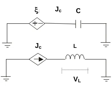
Figure 1. Basic cell of the network model

i-

∆

Jγ=VL

R

R

i

i+

∆

ξξ

J

_C

J

V

connecting a current source in the node that correspond to that end. Figure 3 shows the network model with these boundary conditions, where each cell is given by Figures 1 and 2, and F(t) is the force applied at the beginning of the rod. We have found the response to three different forces F(t): a step pulse (Figure 4), a low-frequency harmonic force (Figure 5) and a high-frequency harmonic force (Figure 6). We have compared it with the analytical solution obtained by using the techniques shown in [5]. In order to have general results, dimensionless variables have been used.

The step pulse have a duration of 0.05 s, the frequencies of the harmonic forces are 25 Hz and 25 kHz, and all the forces have a dimensionless amplitude of 1. The rod is made with aluminium having phase velocity c=5150 m/s and Young´s modulus Y=7.1x1010 N/m.

Figure 4. Response at the central point of the forced-fixed rod to a step pulse.

Figure 5. Response at the central point of the forced-fixed rod to a low-frequency harmonic force (25 Hz).

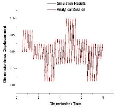
Figure 6. Response at the central point of the forced-fixed rod to a high-frequency

harmonic force (25kHz).

X=0

X=L

r

F(t)

Forced-Free Rod

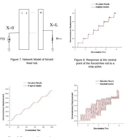
The response of a rod with a free end and an external force applied at the beginning of the rod, x=0, have also been simulated. The boundary condition of free end is incorporated to the network model connecting an infinite resistance to the node that corresponds to that end, so the current in that branch is zero. Figure 7 shows the network model with these boundary conditions. Again, the response of the rod to three different forces have been found: a step pulse (Figure 8), a low-frequency harmonic force (Figure 9) and a high-frequency harmonic force (Figure 10), and we have compared it with the analytical solution.

Figure 8. Response at the central point of the forced-free rod to a

step pulse.

Figure 9. Response at the central point of the forced-free rod to a low-frequency harmonic force (25 kHz)

Figure 10. Response at the central point of the forced-free rod to a high-frequency harmonic force (25 kHz).

X=0

X=L

F(t) R=∞

It can be seen from these figures that the displacement in the forced-free rod increases throughout the time. It is due to the mathematical model which we have considered, but when the displacement is very high the equation (1) is not valid and it is necessary to use a more complicated model.

CONCLUSIONS

The comparison between the results obtained from the simulation and the analytical solution of the response of the two kinds of rod (forced-fixed and forced-free) to every external force shows that all the simulations have results very similar to the analytical solutions (in the case of harmonic force of low frequency are nearly identical). It can be seen that the simulations present errors when the solution changes very fast, however they are small and shows a very high agreement with the theoretical solution.

These results show that this simulation method can be applied to more complicated and practical cases without analytical solution (or very difficult to obtain), as the case of a rod with a mass at the end of the road [1] [5], or including the dumping and/or dispersion of the wave [5].

REFERENCES

[1] Kinsler L, Frey A, Coppens A, Sanders J, “Fundamentos de Acústica” Editorial Limusa, Mexico, 1992.

[2] Horno J., García-Hernandez M. T., Gonzalez-Fernández C. F., J. Electroanal. Chem., 377 (1994) 53.

[3] MicroSim Pspice, Version 8. Microsim Corporation. 1996.

[4] Nagel L. W., SPICE2: A computer program to simulate semiconductor circuits, Ph. D. Thesis, Memo. UCB/ERL M520, University of California, Berkeley, CA, 1977.

[5] Graff K. L., “Wave Motion in Elastic Solids” Dover Publications, U.S.A., 1991.

ACKNOWLEDGMENTS