Finance, growth, and institutions in Latin America : what are the links?
30
0
0
Texto completo
(2) 180. LATIN AMERICAN JOURNAL OF ECONOMICS | Vol. 50 No. 2 (Nov, 2013), 179–208. through pooling the savings of individuals, resulting in specialization and greater capital accumulation and productivity.2 Although there is a vast amount of work on the finance-growth link, there is no consensus on how financial development af fects economic growth. While several theoretical and empirical analyses show that financial development leads to economic growth (Beck, Levine, and Loayza, 2000; Rajan and Zingales, 2003), some provide evidence that financial development has no significant effect on economic growth (Shan, 2005). Others argue that the ef fect is dependent on certain conditions (Rioja and Valev, 2004a,b) and that financial development may have a negative ef fect in some cases, depending on the time frame considered (Loayza and Ranciere, 2006). Thus, the study of the finance-growth link continues to be a topic of interest. There is also a growing body of work on the factors that explain financial development. This paper studies the impact of financial development on economic growth in the short and long run and the determinants of financial development in Latin America. This analysis contributes to the literature in several ways. First, it expands on Loayza and Ranciere’s (2006) study of the impact of financial development on economic growth by focusing only on the Latin American region and expanding the sample period. Second, along the lines of the work of Rioja and Valev (2004a), this analysis considers different income groups when determining the long- and short-term effect of financial development on economic growth. Third, in relation to the study of the determinants of financial development, this paper expands on the work of Chin and Ito (2006) and Baltagi et al. (2009) by focusing on Latin American countries, expanding the sample period, and considering other factors related to institutions and country stability as possible determinants of financial development. This paper answers the following questions for the Latin American region: 1) What is the ef fect of financial development on economic growth for dif ferent time frames and across countries with varying income levels? 2) What factors lead to greater financial development? Studying financial development in Latin America is relevant for several reasons. First, countries in Latin America share a common set of coef ficients due to their shared experience, which is not necessarily the case for other regions (Grier and Tullock, 1989). Second, Latin America 2. Please refer to Levine’s (1997) work for a more in-depth discussion of the individual functions performed by the financial sector. Levine also provides a good parable that provides a complete understanding of the key role that the financial sector plays in the economy..
(3) Luisa Blanco | FINANCE, GROWTH, AND INSTITUTIONS IN LATIN AMERICA. 181. is a natural laboratory for studying the impact and determinants of financial development because the region has experienced significant improvements in the financial sector in the last decades. Thus, there is significant variation over time. Third, there is suf ficient variation in our variable of interest, financial development, across countries in the region. For example, in the 1970-1974 period, while private credit as a share of GDP is 27% for Mexico, it is only 6% for Bolivia. Then, in the 2006-2010 period, Panama shows the highest level of private credit as a share of GDP (78%), while Argentina is at the bottom (12%). Using data for the 1961-2010 period in a panel framework for 16 Latin American countries, the main findings in relation to the impact of financial development on economic growth are the following. For the full sample, financial development has a significant positive effect on economic growth in the long run, but a significant negative effect in the short run. This finding agrees with the conclusions of Loayza and Ranciere (2006). Nonetheless, we find that countries in the region do not share the same set of coefficients, such that the long-run positive effect of financial development on economic growth only holds for the high-income group. For the low-income group, financial development has a significant negative effect in the long run. Financial development has no significant effect on economic growth in the short run for either the high- or low-income group. In the analysis of the determinants of financial development, using 5-year average observations during the period 1985-2010, greater financial openness and lower country risk are associated with greater financial development. Financial openness seems to create the most significant benefit in those countries that are relatively closed. Of the components of the country risk index (financial, economic, and political), the financial risk index has a positive significant effect, while the economic risk index has a negative significant effect. Of the components of the financial risk index, the index related to foreign debt is positive and statistically significant (lower foreign debt as a share of GDP is associated with greater financial development). Of the components of the political risk index, only the socioeconomic conditions index has a positive significant effect on financial development at the 5% level, while the indices related to internal conflict, government stability, and investment profile are positive and marginally statistically significant (10% level). None of the components of the economic risk index show a significant effect. This paper is organized as follows. Section 2 presents a brief review of literature on the finance-growth link and the determinants of financial.
(4) 182. LATIN AMERICAN JOURNAL OF ECONOMICS | Vol. 50 No. 2 (Nov, 2013), 179–208. development, and Section 3 describes the methodology. Sections 4 and 5 present the results and a discussion of sample issues and main findings, respectively. Section 6 concludes.. 2.. Literature review. 2.1. The finance-growth link While the general belief is that financial development has a positive ef fect on economic growth (supply-leading hypothesis), there is theoretical and empirical work indicating that this effect is non-existent and that financial development is merely a consequence of economic growth (demand-following hypothesis).3 Financial development can be generally defined as increasing access to credit, and the positive ef fect of financial development on growth is derived from the ef fect financial development has on capital accumulation and productivity (Beck, Levine, and Loayza, 2000). With the development of the financial sector comes greater access to capital that results in more funding available for attractive investment opportunities. Greater access to capital leads to increased labor specialization and more access to new technology (Rajan and Zingales, 2003; Saint-Paul, 1992). Consequently, improvements in capital markets lead to greater economic growth. On the other hand, there has been some questioning of the benefits derived from financial development. There are three main reasons to be skeptical about the impact of financial development on economic growth. First, there is research that supports the demandfollowing hypothesis, where financial development is a consequence of economic growth (Shan, 2005). Second, the impact of financial development on economic growth seems to be dependent on certain conditions. There is empirical evidence showing that the ef fect of financial development on growth is dif ferent across regions and among countries with dif ferent income levels, levels of financial development, and institutional frameworks (see Aghion et al., 2005; Blanco, 2009; De Gregorio and Guidotti, 1995; Rioja and Valev, 2004a,b; and Shen and Lee, 2006, among others). Third, financial development can produce greater macroeconomic volatility, becoming a destabilizing force in the economy (Loayza and Ranciere, 2006). 3. Refer to Blanco (2009) and Levine (2005) for a thorough discussion of the literature on the financegrowth link. Odhiambo (2007) presents a good discussion on the supply-leading and demand-following hypotheses..
(5) Luisa Blanco | FINANCE, GROWTH, AND INSTITUTIONS IN LATIN AMERICA. 183. When financial development leads to volatility, it is expected that financial development will have a negative ef fect on economic growth. According to Loayza and Ranciere (2006), the short-run ef fect of financial development on economic growth may be negative due macroeconomic instability, but the long-run ef fect is expected to be positive. Thus, looking at the impact of financial development at dif ferent time frames is necessary. In the Latin American context, where countries have experienced periods of volatility, distinguishing the short- and long-run effect of financial development is of special interest to policymakers. When studying the impact of financial development on economic growth, it is also important to keep in mind that financial development might have a differential impact on growth depending on specific country conditions. Some countries will be better equipped to absorb the influx of credit. It is likely that specific country characteristics, in relation to their level of development (i.e., income) could determine a country’s ability to use the influx of credit productively. For this reason, studying the impact of financial development for countries with different income levels is relevant for the design of future policies related to financial markets in Latin America.. 2.2. Sources of finance In the review of the literature, the factors considered to be the main determinants of financial development are the degree of openness, institutions, and political stability. Liberalization of goods and capital markets are associated with greater financial development (Baltagi et al., 2009; Chinn and Ito, 2006; Klein and Olivei, 2008). Openness to trade and capital flows have been proposed as important determinants of financial development. According to Rajan and Zingales (2003), there will be interest groups who will oppose financial development due to the competition it brings. With trade and financial liberalization, the power of those groups opposed to financial development is significantly weakened. Therefore, substantial financial reforms can take place when the power of such interest groups is diminished by openness, leading to greater financial development. Financial liberalization is associated with the strengthening of the financial system in two ways.4 First, as a result of financial 4. Refer to Chinn and Ito (2006) and Klein and Olivei (2008) for a comprehensive literature review of the channels through which financial liberalization leads to greater financial development..
(6) 184. LATIN AMERICAN JOURNAL OF ECONOMICS | Vol. 50 No. 2 (Nov, 2013), 179–208. liberalization, the entrance of foreign banks into the domestic financial sector leads to an increase in available loanable funds and ef ficiency. Ef ficiency in the financial sector increases significantly with financial liberalization since there is greater competition and more pressure to reform the financial sector. Second, Klein and Olivei (2008) argue that a virtuous cycle of greater savings and ef ficiency is created with increasing capital account openness because financial intermediaries are able to achieve economies of scale. Furthermore, institutions seem to play a key role in explaining differences in financial development across countries.5 According to Chinn and Ito (2006), there are two dif ferent categories of institutions that have been considered important determinants of financial development: 1) institutions that affect the economy as a whole, and 2) institutions that af fect the financial sector.6 In the first group, the relevant institutions are related to bureaucratic quality, law and order, and control of corruption, among others. Because these institutional factors directly af fect the way business is done and relate to perceptions about the stability of the legal system, they are expected to be associated with greater levels of financial development. The second group of institutions includes those that specifically af fect the financial sector. According to Djankov et al. (2007), institutions that increase creditor power and access to lending information are crucial for financial development. When creditor rights are enforced, credit is likely to expand because creditors feel more protected against default. Creditors are also more likely to lend when they are able to get more information about potential lenders. Greater financial depth is expected when there is an increase in access to information on borrowers and protection for private credit institutions. Furthermore, the stability of a specific country may significantly influence capital markets. The degree to which there is stability in a country af fects investors’ perceptions and consequently their willingness to invest in that country. According to Roe and Siegel (2009), a country’s capacity to protect investors is related to political 5. Beck and Levine (2005) present an excellent review of the literature on the relationship between institutions and financial development. 6. Here we follow the categorization provided by Chinn and Ito (2006) to distinguish the dif ferent types of institutions. Other institutions related to the financial sector could be those that help to promote stability in the financial sector. Institutions that help promote stability are likely to be related to the design and enforcement of prudent regulations. Data about these types of institutions are unlikely to be available consistently over time for the sample used in this analysis..
(7) Luisa Blanco | FINANCE, GROWTH, AND INSTITUTIONS IN LATIN AMERICA. 185. stability. Thus, countries with unstable political systems of fer low protection to investors. Empirical evidence on the importance of openness and institutions as factors explaining financial development is abundant. The crosssectional analysis by Herger et al. (2008) shows that trade openness has a significant ef fect on financial development. In a panel framework that includes only less developed countries, Baltagi et al. (2009) find that trade and financial openness are relevant to explaining financial development. They investigate the interactions between trade and financial openness and find that this interaction term is negative. They conclude that while financial development requires both types of openness, relatively closed economies benefit the most from opening up to trade or capital. Chinn and Ito (2006) find that at a certain institutional threshold, financial liberalization has a positive ef fect on financial development. Results from Klein and Olivei (2008) are along the lines of Chinn and Ito’s (2006) findings. Klein and Olivei (2008) find that institutions drive the positive ef fect of financial liberalization on financial development, where developed countries that have better institutions obtain greater benefits from financial liberalization. The openness to trade and capital flows experienced during the process of globalization are likely to be associated with institutional reforms that significantly af fect capital markets (Mishkin, 2009). There is also empirical evidence regarding the impact of institutions and political stability on financial development. Acemoglu and Johnson (2005) find that institutions that af fect all sectors of the economy have a significant direct ef fect on financial development. They show empirically that property rights and contracting institutions are important determinants of financial development. Beck et al. (2003) also find that institutions, shaped by either legal origins or initial resource endowments, have a significant ef fect on financial development in a sample of 70 former colonies. Andrianova et al. (2008) report evidence that institutions related to governance have a significant ef fect on financial development, where lower quality of institutions is associated with greater government ownership in the financial sector. In relation to institutions that af fect capital markets, Djankov et al. (2007) present strong empirical evidence that creditor rights and access to lending information are important determinants of financial development. Additionally, Roe and Siegel (2009) present empirical evidence showing that political instability explains financial backwardness..
(8) 186. LATIN AMERICAN JOURNAL OF ECONOMICS | Vol. 50 No. 2 (Nov, 2013), 179–208. While there are several papers on the determinants of financial development, few have taken a regional approach. When studying the factors that lead to greater financial depth, it is important to focus on countries with a common historical, political, and socio-economic background. It is unlikely that the factors that explain financial development in a specific country in Asia or Africa would explain capital markets in Latin America. By taking a regional approach to the study of the sources of finance, more specific policy recommendations could be provided.. 3.. Methodology. 3.1. Impact of financial development on economic growth In studying the impact of financial development on economic growth in the short and long run for Latin America, this analysis follows the methodology of Loayza and Ranciere (2006) closely. Loayza and Ranciere (2006) propose using the pooled mean group (PMG) estimator developed by Pesaran et al. (1999).7 For the PMG estimator, an autoregressive distributive lag (ARDL(p,q,q,…,q)) dynamic panel specification is applied. A vector error correction model (VECM) is considered under this specification, where the short-run dynamics of the variables in the system are influenced by the deviation from equilibrium. The ARDL(p,q,q,…,q) used for the PMG estimator is specified as follows:. yit =. p. q. j =1. j =0. ∑ λij yi,t −j + ∑ δij' Χi,t −j + µi + εit. (1). where yit represents the dependent variable for t = 1, 2,…,T time periods, and i = 1, 2, …, N groups. Xi,t ‒ j is the k x 1 vector of explanatory variables (regressors) for group i, δij are k x 1 coef ficient vectors, λij are scalars, µi represents the fixed ef fect, and εit the time varying disturbance. Equation (1) can be reparametrized in the following way and time series observations for each group are stacked. 7. Refer to Loayza and Ranciere (2006) for an explanation of the appropriateness of the PMG estimator when disentangling the finance-growth link and a description of this methodology. Refer also to Blackburne and Frank (2007) for a description of the PMG estimator in Stata..
(9) Luisa Blanco | FINANCE, GROWTH, AND INSTITUTIONS IN LATIN AMERICA. 187. p −1. ∆yi = φi yi,−1 + Χi βi + ∑ λij* ∆yi,− j q −1. +∑. j =1. j =1. ∆Χi,− j δij*. (2). + µi ι + εi. where yi is a t x 1 vector of the observations of the dependent variable of the ith group, Xi is a t x k matrix of the regressors that vary across groups and time periods, and ι is a t x 1 vector of 1s. One of the main requirements of this model’s specification is the existence of a long-run relationship between yit and Xit, where the error-correcting speed of adjustment term for the long-run relationship represented by φi must be significantly negative (and no lower than -2). The long-run relationship between yit and Xit for each group is expressed as follows:. yit = −(βi' / φi )Χit + ηit. (3). where η is a stationary process. For the long-run homogeneity assumption, the coefficients on Xi are the same across groups. Longrun coef ficients of Xi are expressed as θi = −βi/φi, where θi = θ. In the PMG estimator, while the long-run coef ficients are equal across groups, the intercept, short-run coef ficients, and error variances dif fer across countries.8 For the PMG estimation in this analysis, real GDP growth (first dif ference of the natural log of real GDP per capita) is the dependent variable and financial development (private credit in natural logs) is in the right-hand side of the equation.9 Initial GDP per capita (natural log), government size (natural log), trade, and inflation are included as control variables.10 A dynamic specification of the form ARDL(3,3,1,1,1,1) is used, and all variables are time-demeaned.11 All 8. See Blackburne and Frank (2007) for a good explanation of the specification of the PMG model. Asteriou and Hall (2007) also provide a brief discussion of the PMG estimator. 9. The methodology used here, following Loayza and Ranciere (2006, p. 1055), addresses the two-way causality between financial development and economic growth. One of the conditions for validity is that “the dynamic specification of the model be suf ficiently augmented so that the regressors are strictly exogenous and the resulting residual is serially uncorrelated.” 10. These variables are constructed following the approach of Loayza and Ranciere (2006); refer to Table A1 for a description of how these variables were constructed. 11. Lag lengths selected based on the augmented Dickey-Fuller (ADF) regressions. The number of lags is selected in such a way that the Akaike information criterion (AIC) for the regression is minimized. This process is carried out for each panel. The PMG estimator provides consistent estimators when the variables are I(0) and I(1), so there is no need to include unit root tests in the analysis..
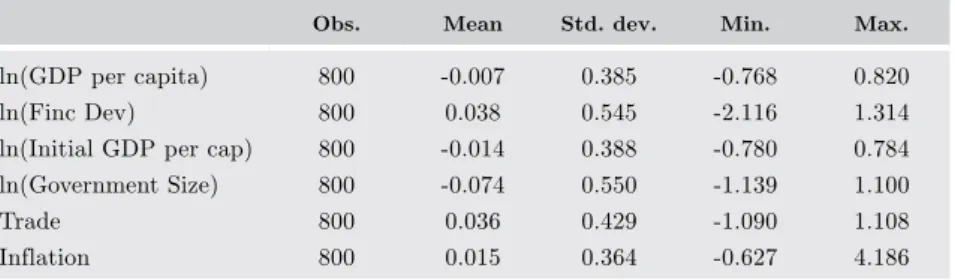
(10) 188. LATIN AMERICAN JOURNAL OF ECONOMICS | Vol. 50 No. 2 (Nov, 2013), 179–208. independent variables are entered in levels for the long-run relationships and in first dif ference for the short-run relationships. The ARDL form specified above includes the first and second lag of the first dif ference of real GDP and private credit as regressors. Annual observations between 1961 and 2010 are used for this part of the analysis. Because of the lag structure of the model, estimations will include observations between 1964 and 2010 (47 observations per country). Table 1 shows the summary statistics, and Table 1 in the appendix provides a description of the variables used and their sources.. 3.2. Determinants of financial development In this analysis, the approach taken to find out what factors explain financial development in Latin America is similar to the one used by Baltagi et al. (2009). The dynamic panel general method of moments (GMM) suggested by Arellano and Bond (AB, 1991) is implemented and an ARDL(p,q,q,…,q) specification is considered for the AB estimator. For the AB estimator, the first lag of the dependent variable is included in the right-hand side of the equation, which leads to endogeneity issues since the lag of the dependent variable is determined by the error term. This endogeneity problem biases the estimates provided by the general GMM. Arellano and Bond (1991) propose differencing the data to address the endogeneity of the variables on the right-hand side and control for specific country characteristics.12 The Arellano and Bond (1991) GMM uses lagged levels of the dependent variable as instruments to address the endogeneity of the dependent variable. The model specification of the AB estimator can be expressed as:. ∆yit = ρ∆yi,t −1 + ∆Χit βi + ∆εit. (4). Equation (4), which represents first dif ference transformation and removes the constant term and individual effects, shows that the lag of the dependent variable is included as a regressor and Xit is the tN x k matrix of the explanatory variables. For this estimation, the instruments used are the available lags of the levels of the endogenous variables.. 12. Using Arellano and Bond’s GMM estimator allows us to see the ef fect of the factors considered as determinants of financial development when addressing endogeneity. This methodology requires us to take the first dif ference of the dependent variable, which can be interpreted as the growth of finance, thus enabling us to see whether the independent variables are associated with changes in financial development in Latin America..
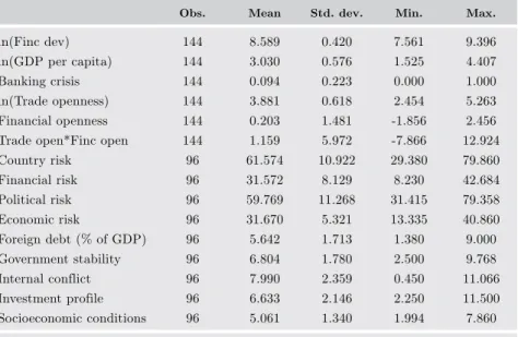
(11) 189. Luisa Blanco | FINANCE, GROWTH, AND INSTITUTIONS IN LATIN AMERICA. Table 1. Impact of financial development on growtha (summary statistics) Obs.. Mean. Std. dev.. Min.. Max.. ln(GDP per capita). 800. -0.007. 0.385. -0.768. 0.820. ln(Finc Dev). 800. 0.038. 0.545. -2.116. 1.314. ln(Initial GDP per cap). 800. -0.014. 0.388. -0.780. 0.784. ln(Government Size). 800. -0.074. 0.550. -1.139. 1.100. Trade. 800. 0.036. 0.429. -1.090. 1.108. Inflation. 800. 0.015. 0.364. -0.627. 4.186. a. Annual observation, 1961-2010, 16 countries (statistics on time-demeaned data).. The methodology of Arellano and Bond (1991) is appropriate for datasets with many panels and few periods. For this reason, and to smooth out short-run fluctuations in the data, five-year average observations are considered in this part of the analysis. These fiveyear average observations are constructed using available data for the period from 1985 to 2010.13 Financial development growth (the first dif ference of private credit as a share of GDP in natural log) is used as the dependent variable, and its first lag is entered in the right-hand side of the equation. The growth of real GDP per capita (first dif ference of real GDP per capita in natural log) and a dummy for the banking crisis are included as control variables.14 The variables of interest that are entered in the right-hand side of the equation are trade openness (natural log), financial openness, the interaction between trade and financial openness, and the country risk index.15 The country risk index is a composite indicator of political,. 13. Five-year averages are based on available data for the periods 1985-89, 1990-94, etc. 14. Note that private credit and real GDP are entered in first dif ference initially as we are interested in considering the relationship between the growth rates of these variables. It is also important to note that the methodology used here allows for dealing with the two-way causality between finance and growth since this estimation method “is suited to panel data, deals with a dynamic regression specification, controls for unobserved time- and country-specific ef fects, and accounts for some endogeneity in the explanatory variables.” (Loayza and Ranciere, 2006: 1067) 15. This analysis focuses on testing empirically the ef fect of financial openness on financial development, which is related to the liberalization of the capital account. Financial liberalization is defined by Ranciere et al. (2008) as the deregulation of domestic financial markets, in addition to liberalization of the capital account. Financial openness and financial liberalization terms are used interchangeably in the literature, but it is important to make the distinction when performing empirical analyses. For example, Abiad and Mody (2005) and Abiad et al. (2008) construct an index of financial liberalization that focuses on financial reform and they present an analysis of the factors explaining it. Chinn and Ito’s (2008) financial openness index, which is used in this analysis, is related only to liberalization of the capital account..
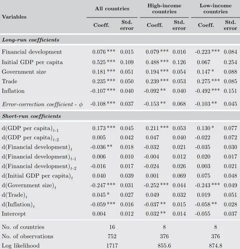
(12) 190. LATIN AMERICAN JOURNAL OF ECONOMICS | Vol. 50 No. 2 (Nov, 2013), 179–208. Table 2. Determinants of financial developmenta (summary statistics) Obs.. Mean. Std. dev.. Min.. Max.. ln(Finc dev). 144. 8.589. 0.420. 7.561. 9.396. ln(GDP per capita). 144. 3.030. 0.576. 1.525. 4.407. Banking crisis. 144. 0.094. 0.223. 0.000. 1.000. ln(Trade openness). 144. 3.881. 0.618. 2.454. 5.263. Financial openness. 144. 0.203. 1.481. -1.856. 2.456. Trade open*Finc open. 144. 1.159. 5.972. -7.866. 12.924. Country risk. 96. 61.574. 10.922. 29.380. 79.860. Financial risk. 96. 31.572. 8.129. 8.230. 42.684. Political risk. 96. 59.769. 11.268. 31.415. 79.358. Economic risk. 96. 31.670. 5.321. 13.335. 40.860. Foreign debt (% of GDP). 96. 5.642. 1.713. 1.380. 9.000. Government stability. 96. 6.804. 1.780. 2.500. 9.768. Internal conflict. 96. 7.990. 2.359. 0.450. 11.066. Investment profile. 96. 6.633. 2.146. 2.250. 11.500. Socioeconomic conditions. 96. 5.061. 1.340. 1.994. 7.860. a. 5-year average observations, 1970-2010, 16 countries. financial, and economic risk indices. Thus, the model is estimated by including the components of the country risk index.16 We also estimate the model with the components of the economic, financial, and political risk indices. In the model specification shown in Equation (4), the first dif ference is taken from all variables to transform the equation into the dif ference GMM. The lagged levels of financial development growth are used to form GMM-type instruments. Table 2 shows the summary statistics for this part of the analysis, and Table A1 in the appendix provides a description of the variables.. 4.. Results. 4.1. Financial development’s impact on economic growth Table 3 presents the estimates obtained when using the PMG estimator to determine the short- and long-run ef fect of financial development on economic growth for the full sample. The first two columns show the. 16. Refer to Table A1 in the appendix for a description of how the country risk index is constructed and its components..
(13) 191. Luisa Blanco | FINANCE, GROWTH, AND INSTITUTIONS IN LATIN AMERICA. Table 3. Impact of financial development on economic growth (pooled mean group estimator) All countries Variables Coef f.. Std. error. High-income countries Std. error. Coef f.. Low-income countries Std. error. Coef f.. Long-run coef ficients. Financial development. 0.076 *** 0.015. 0.079 *** 0.016. Initial GDP per capita. 0.525 *** 0.109. 0.488 *** 0.126. -0.223 *** 0.084 0.067. 0.254. Government size. 0.181 *** 0.051. 0.194 *** 0.054. 0.147 *. 0.088. Trade. 0.235 *** 0.050. 0.239 *** 0.053. 0.275 *** 0.085. Inflation. -0.107 *** 0.040. -0.092 **. 0.040. -0.492 *** 0.151. Error-correction coefficient - φ. -0.108 *** 0.037. -0.153 **. 0.068. -0.103 **. 0.045. 0.130 *. 0.077. Short-run coef ficients. d(GDP per capita)t -1 d(GDP per capita)t -2. 0.173 *** 0.045. 0.211 *** 0.053. 0.005. 0.042. 0.047. 0.040. -0.022. 0.072. 0.018. -0.032. 0.021. -0.035. 0.030. 0.010. -0.004. 0.012. 0.020. 0.017. d(Financial development)t. -0.036 **. d(Financial development)t -2. -0.016. 0.017. -0.024. 0.026. 0.003. 0.021. 0.040. 0.039. 0.001. 0.069. 0.075. 0.048. d(Government size)t. -0.247 *** 0.031. d(Inflation)t. -0.059 *** 0.016. d(Financial development)t -1 d(Initial GDP per capita)t d(Trade)t Intercept. 0.006. 0.045 * 0.004. 0.027 0.012. -0.252 *** 0.044 0.049. 0.032. -0.243 *** 0.049 0.019. 0.051. -0.037 **. 0.015. -0.058 **. 0.028. 0.032 **. 0.014. -0.055. 0.037. No. of countries. 16. 8. 8. No. of observations. 752. 376. 376. Log likelihood. 1717. 855.6. 874.8. *, **, and *** indicate significance at the 10, 5 and 1% levels, respectively. All estimations include 47 observations per country.. coefficients and the standard errors for the full sample. In this estimation, the long-run coefficients of all control variables are significant at the 1% level. The coef ficients for initial GDP per capita and government size are dif ferent than expected, but trade and inflation have the expected signs. For the short-run estimates, all control variables except for initial GDP per capita and trade are statistically significant at the 5% level. Only the coef ficient sign for initial GDP per capita is unexpected, but it is not statistically significant. The first lag of the dependent variable is positive and statistically significant at the 1% level..
(14) 192. LATIN AMERICAN JOURNAL OF ECONOMICS | Vol. 50 No. 2 (Nov, 2013), 179–208. For the full sample, financial development has a positive significant effect at the 1% level on economic growth in the long run. For the short run, financial development has a negative effect, where only its first difference is statistically significant at the 5% level. The first difference of the first and second lag of financial development have positive and negative coefficients, but they are not statistically significant. The positive and negative effect in the long and short run respectively agrees with the finding of Loayza and Ranciere (2006). The Hausman test was performed to ensure that the PMG estimates are preferred to the ones obtained from the mean group (MG) estimator, where the MG estimator fits the model separately for each group. The Hausman test provides evidence that MG estimates are preferred since it rejects the hypothesis that the difference in coefficients is not systematic for the full sample. Thus, the homogeneity restriction is rejected jointly for all parameters. Following the approaches of Rioja and Valev (2004a) and Blanco (2009), this analysis also evaluates the possibility that the ef fect of financial development is dif ferent across dif ferent income groups. This is also an appropriate approach based on the Hausman test results, which suggest that the PMG is not suitable for the full sample. Based on countries’ real GDP per capita in the middle of the sample period (in 1986), the sample is divided into high- and low-income countries. The countries in the high-income group are Argentina, Colombia, Costa Rica, Mexico, Panama, Peru, Uruguay, and Venezuela. The countries in the low-income group are Bolivia, Chile, Dominican Republic, Ecuador, El Salvador, Guatemala, Honduras, and Paraguay.17 In Table 3, columns 3 and 4 present the coef ficients and standard errors for the high-income group, and columns 5 and 6 show estimates for the low-income group. For the high-income group the signs and significance of most coef ficients stay the same. Financial development shows a significant positive ef fect in the long run at the 1% level, but has no significant ef fect in the short run. In the low-income group, 17. After the division there are eight countries in each group, which is just enough to estimate the PMG. The case of Chile is interesting since it is classified as low-income in this study based on 1986 income levels, even though Chile today has one of the highest income levels in the region. Classifying the countries in two income groups rather than three (high-, middle-, and low-income, as Blanco (2009) does) is somewhat restrictive in this set-up, but it is necessary to maintain the properties of the PMG estimator since splitting the sample into three categories would result in a very small sample size when estimating the model for each group. Using the income levels in the middle of the sample when classifying countries provides us with a more consistent classification that is not biased by a posteriori knowledge. Interestingly, if we add Chile to the high-income group, we find from the Hausman test that we reject the null hypothesis that the dif ference in coef ficients is not systematic (which is not the case when Chile is excluded from this group). Thus, Chile does not appear to belong to the high-income group when we use the PMG estimator, so keeping it in the low-income group seems appropriate for this study..
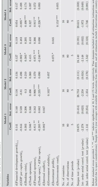
(15) Luisa Blanco | FINANCE, GROWTH, AND INSTITUTIONS IN LATIN AMERICA. 193. the significance and sign of the coef ficients change dramatically. In this estimation, financial development shows a negative significant ef fect in the long run at the 1% level, but no significant ef fect on economic growth in the short run. The Hausman test was performed to ensure that the PMG estimates are preferred to the ones obtained from the MG estimator for the high- and low-income subsamples. We fail to reject the hypothesis that the dif ference in coef ficients is not systematic for both subsamples, which leads us to conclude that the PMG estimates are preferred over the MG estimates. It is also important to note that the condition for the error-correction speed of adjustment is met in all estimations, where φi is statistically significant with a negative value greater than -2.18. 4.2. Determinants of financial development Tables 4 and 5 contain estimates of the model of determinants of financial development in Latin America. In Table 4, the first two columns show the coefficients and standard errors for the baseline model that includes the composite risk index, which accounts for economic, financial, and political risk. Higher values of this index represent lower risk, more stability, and a better institutional environment. All estimations in this section include time dummies, but these estimates are not included due to space considerations. In this estimation, real GDP growth has a negative, marginally significant ef fect at the 10% level, which was unexpected. Banking crisis has a positive, marginally significant ef fect at the 10% level, and its sign was also unexpected. One possible reason for the positive sign of this coef ficient is that this indicator may capture the period of time in which financial sector restructuring takes place. It is dif ficult to detangle the ef fect of the banking crisis dummy since a dummy in a five-year period could account for the pre- and post-crisis period. Trade openness has a positive sign, but it is not statistically significant, which was unexpected. Financial openness and the interaction term between financial and trade openness are significant at the 5% level. While the coef ficient for financial openness has a positive sign, its interactive term with trade openness is negative. This finding agrees 18. The positive coef ficient of initial GDP per capita is unexpected according to convergence theory, and this is noted in the paper. However, this should not af fect the stability of the model since initial GDP per capita is entered as an exogenous variable in the model and the condition for the error-correction speed of adjustment is met in all estimations..
(16) -2.160. -1.398. 2nd-order serial correl. test (p-value). (0.16). (0.03). (0.36). 0.015. Model 2. -1.563. -2.396. 24.672. 5. 80. 16. 0.013. 0.041 ***. -0.043 ***. -0.220 ***. 0.887 ***. 0.650 *. 0.407 *. -1.001 *. 0.046. Coef f.. (0.12). (0.02). (0.17). 0.011. 0.010. 0.015. 0.076. 0.316. 0.358. 0.209. 0.605. 0.124. Std. error. Model 3. -1.491. -2.262. 23.100. 5. 80. 16. 0.165 ***. -0.199 **. 0.797 **. 0.159. 0.432 **. -1.382 **. 0.006. Coef f.. (0.14). (0.02). (0.23). 0.041. 0.086. 0.355. 0.395. 0.177. 0.537. 0.130. Std. error. Robust standard errors provided. *, **, and *** indicate significance at 10, 5 and 1% levels, respectively. Time dummies included in all estimations (estimations not included due to space considerations). Sample uses 5-year averages with available observations from 1981-2010, and all estimations include 5 observations per country.. 20.545. 1st-order serial correl. test (p-value). 5. Sargan test (p-value). 80. No. of time periods. 16. 0.027 *. 0.087. 0.364. -0.193 **. 0.757 **. 0.201. 0.367 * 0.351. 0.614. 0.432. 0.114. Std. error. 0.130. Model 1. -1.154 *. Coef f.. No. of observations. No. of countries. d(Foreign debt)t. d(Political risk)t. d(Financial risk)t. d(Economic risk)t. d(Country risk)t. d(Trade open)t * d(Finc open)t. d(Financial openness)t. d(Trade openness)t. d(Banking crisis)t. d(GDP per capita growth)t. d(Financial development growth)t -1. Variables. (Arellano and Bond estimator). Table 4. Sources of financial development. 194 LATIN AMERICAN JOURNAL OF ECONOMICS | Vol. 50 No. 2 (Nov, 2013), 179–208.
(17) -2.278. -1.141. 1st- order serial correl. test (p-value). 2nd- order serial correl. test (p-value). (0.254). (0.023). (0.414). 0.047. 0.082. 0.342. 0.346. -1.354. -2.258. 26.753. 5. 80. 16. 0.102 *. -0.235 ***. 0.966 ***. 0.496. 0.3. -0.81. 0.116. (0.176). (0.024). (0.111). 0.057. 0.090. 0.370. 0.360. 0.210. 0.496. 0.134. Std. error. Model 2 Coef f.. 0.127. -1.542. -2.148. 24.140. 5. 80. 16. 0.075 *. -0.240 ***. 0.971 ***. 0.415. 0.383 *. -0.902 *. (0.123). (0.032). (0.191). 0.045. 0.090. 0.366. 0.410. 0.205. 0.483. 0.119. Std. error. Model 3 Coef f.. 0.054. -1.746. -1.972. 20.615. 5. 80. 16. 0.153 ***. -0.226 **. 0.915 **. 0.327. 0.490 ***. -0.895 *. (0.081). (0.049). (0.359). 0.055. 0.093. 0.372. 0.397. 0.174. 0.498. 0.117. Std. error. Model 4 Coef f.. Robust standard errors provided. *, **, and *** indicate significance at 10, 5 and 1% levels, respectively. Time dummies included in all estimations (estimations not included due to space considerations). Sample uses 5-year averages with available observations from 1981-2010, and all estimations include 5 observations per country.. 19.675. 5. No. of time periods. Sargan test (p-value). 16. 80. No. of countries. 0.082 *. -0.205 **. 0.811 **. 0.586 *. 0.206. 0.539. 0.303. 0.140. 0.141. -0.844. Std. error. Model 1. Coef f.. No. of observations. d(Socioeconomic cond)t. d(Investment profile)t. d(Government stability)t. d(Internal conflict)t. d(Trade open)t * d(Finc open)t. d(Financial openness)t. d(Trade openness)t. d(Banking crisis)t. d(GDP per capita growth)t. d(Financial development growth)t -1. Variables. (Arellano and Bond estimator). Table 5. Sources of financial development. Luisa Blanco | FINANCE, GROWTH, AND INSTITUTIONS IN LATIN AMERICA. 195.
(18) 196. LATIN AMERICAN JOURNAL OF ECONOMICS | Vol. 50 No. 2 (Nov, 2013), 179–208. with Baltagi et al. (2009). The negative coef ficient of the interaction term implies that the effect of capital openness on financial development will be greater for relatively closed economies than for relatively open economies. The country risk index has a positive sign and is marginally significant at the 10% level. From the estimates shown in Table 4, it is apparent that the lag of the dependent variable is not statistically significant. This raises the question of whether the dynamic model panel approach, where the lagged dependent variable is included as a regressor, is the adequate model. A lag length test provides evidence that one lag of the financial development growth indicator is the adequate number of lags.19 In Table 4, columns 3 and 4 (Model 2) provide the estimates obtained when the components of the country risk index (economic, financial, and political risk indices) are included. These estimates show that only the economic and financial risk indices have a significant ef fect on financial development at the 1% level. While the economic index has a negative sign, the financial index has a positive sign. This suggests that a decrease in financial risk (higher index value) is beneficial for financial development, but a decrease in economic risk (higher index value) is detrimental to financial development. The ef fect of the economic index on financial development was not predicted, as more stable economic conditions would be expected to be more conducive to expansion of the financial sector. We explore whether the components of the three dif ferent indices have a significant ef fect on financial development, and estimate our model, examining each component one at a time to avoid multicollinearity issues. We estimated our model 22 times (the economic risk index has five components, as does the financial risk index, while the political risk index has 12), and include in our tables those estimations where we find that the components of the indices are statistically significant at least at the 10% level.20 We provide a description of the variables that compose these indices and were statistically significant in our estimations in the Appendix (Table A1).21. 19. Lag length selected using the ADF regressions, where the regression that minimizes the AIC is chosen (in a panel set-up). 20. Other estimations that include the other components of the risk indices, one at the time, are not included for space considerations but are available from the author upon request. 21. Please refer to the Political Risk Group website for a discussion of the 22 variables that compose the dif ferent risk indices (http://www.prsgroup.com/ICRG_methodology.aspx)..
(19) Luisa Blanco | FINANCE, GROWTH, AND INSTITUTIONS IN LATIN AMERICA. 197. The economic index measures a country’s economic strengths and weaknesses and is composed by indices of GDP per capita, economic growth, inflation rate, budget balance as a percentage of GDP, and current account as a percentage of GDP. We find that none of these components were statistically significant in our model. The financial risk index indicates the ability of a country to meet its financial obligations, such as of ficial, commercial, and trade debt obligations. This index is composed of several indices that are related to foreign debt as a percentage of GDP, foreign debt service as a percentage of exports of goods and services, current account as a percentage of exports of goods and services, net international liquidity as months of import cover, and exchange rate stability. From these indices, interestingly, only the index related to foreign debt as a percentage of GDP was statistically significant. Columns 5 and 6 in Table 4 (Model 3) show the estimates obtained when we include the index related to foreign debt as a percentage of GDP, which is positive and statistically significant at the 1% level. A decrease in foreign debt as a percentage of GDP is associated with a higher index, and consequently with a higher level of financial development. The model specified in Equation (4) is also estimated using the 12 components of the political risk index, one at a time. The components of the political risk index, which are closely related to institutions and country stability, are the following: government stability, socioeconomic conditions, investment profile, internal conflict, external conflict, corruption, military in politics, religious tensions, law and order, ethnic tensions, democratic accountability, and bureaucratic quality. The indicators that account for institutions that af fect the economy as a whole and that are included in the political risk index are corruption, law and order, and bureaucratic quality. The investment profile index is the indicator that accounts for institutions that directly af fect the financial sector since it is composed of indicators related to contract viability, expropriation, profits repatriation, and payment delays. A close relationship is expected between the investment profile index and our financial development indicator since the investment profile is related to investment risk and consequently to the willingness to invest in a specific country. Thus, there is important feedback between these two indicators, and it is expected that the AB estimator will allow for estimating the independent ef fect of financial sector institutions on financial development..
(20) 198. LATIN AMERICAN JOURNAL OF ECONOMICS | Vol. 50 No. 2 (Nov, 2013), 179–208. Four components are statistically significant when the model is estimated by including each component of the political risk index one at a time; the estimations are shown in Table 5. In that table, internal conflict (columns 1 and 2), government stability (columns 3 and 4), and investment profile (columns 5 and 6) have a positive significant ef fect on financial development at the 10% level. The index of socioeconomic conditions is positive and statistically significant at the 1% level (Table 5, columns 7 and 8). This index measures the degree to which socioeconomic pressures related to unemployment, consumer confidence, and poverty constrain government actions or fuel social dissatisfaction.22. 5.. Discussion. In relation to the sample used in this analysis, which is restricted to 16 Latin American countries, we consider the possibility of expanding our sample to include three other countries for which there is consistent financial development data available during the period of analysis: Jamaica, Haiti, and Trinidad and Tobago. However, because we believe that these countries do not share the same historical legacy and socioeconomic background as the countries included in the main sample, we did not initially include them in the main estimations. The excluded countries are also not Spanish-speaking countries. Trinidad and Tobago is classified as a high-income economy by the World Bank, where all the other countries in our sample are classified as developing countries.23 Although Jamaica, Haiti, and Trinidad and Tobago generally cannot be considered developing Latin American countries, we explore their inclusion in the estimations performed in this analysis. We estimate the model specified in Equation (2), which estimates the long- and short-run ef fect of financial development on economic growth using the PMG and including these three countries. We find that when these countries are included in the full sample, financial development continues to have a positive ef fect on economic growth in the long run 22. Note that in all the estimations the Sargan test shows that the instruments used are adequate since the hypothesis that the overindentifying restrictions are valid is not rejected. The serial correlation tests also show that the idiosyncratic errors are independently and identically distributed (i.i.d.) as required for the AB estimation. In all AB estimations we also meet the conditions of rejecting first-order autocorrelation and not rejecting the second-order autocorrelation at the 5% level. 23. We refer to the latest country classification provided by the World Bank (http://data.worldbank. org/about/country-classifications/country-and-lending-groups#LAC)..
(21) Luisa Blanco | FINANCE, GROWTH, AND INSTITUTIONS IN LATIN AMERICA. 199. at the 1% level, and the coefficient is of the same magnitude as is shown in Table 3, column 1. We also find that financial development has a significant negative ef fect in the short run, where the coef ficient of the first dif ference of private credit is negative and statistically significant at the 1% level, and of the same magnitude as before. Nonetheless, we find in the Hausman test that when these countries are included in the estimation, we reject the hypothesis that the PMG estimates are appropriate, which tells us that these countries do not share the same set of coef ficients as the other countries. We also explore whether the results we found in relation to the highand low-income groups are robust to the inclusion of these countries. We again classify countries by their 1986 income level, where Trinidad and Tobago and Jamaica are added to the high-income group and Haiti to the low-income group. The estimations obtained here are very similar to those shown in Table 3. For the high-income group, with the inclusion of these two countries, financial development also has a positive significant ef fect in the long run at the 1% level. For this subsample, the Hausman test tells us that the PMG is preferred over the MG since we reject the hypothesis that the difference in coefficients is not systematic. Thus, based on the Hausman test, excluding these countries from the estimation is appropriate. For the low-income group, when Haiti is added we find that financial development no longer has a significant negative ef fect on economic growth in the long run as was found previously; in this estimation the long-run coef ficient of private credit is positive and statistically significant. For this subsample we find that the PMG is preferred over the MG, but we find that the condition for the error-correction speed of adjustment is not met in this estimation, where φi is positive and statistically insignificant. Thus, we can also conclude here that the inclusion of Haiti in the estimation may not be appropriate. From the estimations related to the ef fect of financial development in the long and short run, we can summarize the main findings as follows. First, the ef fect of financial development on economic growth is different across different income groups. Thus, examining the impact of financial development for the whole region may not be appropriate as countries do not share the same set of coef ficients in relation to the finance-growth relationship. Second, the impact of financial development for the dif ferent subsamples is of small magnitude and varies according to the dif ferent income groups. Using the coef ficients shown in Table 3,.
(22) 200. LATIN AMERICAN JOURNAL OF ECONOMICS | Vol. 50 No. 2 (Nov, 2013), 179–208. column 3, a 1% increase in private credit is associated with a 0.08% increase in economic growth in the long run for the high-income group. For the low-income group, using the coef ficients shown in Table 3, column 5, a 1% increase in private credit is associated with a long-run decrease in economic growth of 0.22%. It is interesting to note that we do not find evidence of short-run ef fects, which goes along with Bangake and Eggoh’s (2011) finding. Our analysis here supports the claim by Bangake and Eggoh (2011) that these countries should focus on implementing long-run policies. We also consider including Jamaica, Haiti, and Trinidad and Tobago in the estimations in which we model the determinants of financial development for Latin American countries. In these estimations, we find similar results to those shown in Tables 4 and 5. The only dif ference is that when including these countries, only the indices related to investment profile and socioeconomic conditions are positive and significant at the 1 and 5% levels, respectively. The index related to foreign debt continues to be positive and statistically significant at the 1% level. Financial openness and its interaction with trade openness are also statistically significant in all these estimations and have the same signs as before. From the estimations related to the determinants of financial development, we can summarize our findings in the following way. First, financial openness has a robust, positive ef fect on financial development, while its interaction with trade openness has a robust, negative significant ef fect. Financial openness seems to be the key player in explaining financial development, which may be because of the sample period used. This analysis encompasses the 1985-2010 period, during which financial markets opened up significantly in Latin America. In fact, the standard deviation for the index of financial openness is more than double the standard deviation of the trade openness indicator. Second, the indices related to foreign debt as a percentage of GDP and socioeconomic conditions seem to be the only indicators that have a positive, significant ef fect on financial development at least at the 5% level. When looking at the magnitude of the ef fect of financial openness on financial development, and taking into consideration the interactive term with trade openness, we find that an increase in the financial openness index of 0.10 point leads to an increase in financial development of 5.64% (using coef ficients in Table 4, column 1), which is of significant.
(23) Luisa Blanco | FINANCE, GROWTH, AND INSTITUTIONS IN LATIN AMERICA. 201. magnitude. In relation to the other variables that were statistically significant at the 5% level, we find that an increase in the foreign debt index (decrease in foreign debt) or an increase in the socioeconomic conditions index (decrease in socioeconomic pressures) of 1 point is associated with an increase on financial development of 17 and 15%, respectively, which is of relevant magnitude.. 6.. Conclusion. In the analysis of the impact of financial development on economic growth, there is one main finding: the impact of financial development on economic growth varies across the Latin American region. This analysis shows that financial development has a positive significant ef fect in the long run only for the high-income group. For the lowincome group, empirical evidence shows that the impact of financial development on economic growth is negative in the long run. The results obtained when the sample is separated by income groups corroborate previous findings that the effect of financial development is dependent on certain conditions. This must be taken into consideration when designing policies to promote economic growth by developing the financial sector in Latin America. Promoting the deepening of financial markets seems to be beneficial for high-income countries, but not for low-income countries. Therefore, financial reform should be a priority for those countries with relatively high income levels in Latin America, but not for all. For further research, disentangling those conditions that allow the relatively high-income group to reap the benefits of financial development in the long run is necessary. Perhaps preconditions related to institutions or a certain financial development threshold might be relevant. In relation to the determinants of financial development in Latin America, financial openness plays a key role in the development of financial markets, where it has a robust, positive, significant ef fect of great magnitude. The analysis here provides evidence that financial openness is the most beneficial in terms of improving financial markets in those countries that are relatively closed. Thus, countries with trade restrictions will find that liberalizing capital accounts can lead to significant expansions of credit. This analysis shows that country risk and some of the components of this index are important sources of financing in the region. Specifically,.
(24) 202. LATIN AMERICAN JOURNAL OF ECONOMICS | Vol. 50 No. 2 (Nov, 2013), 179–208. the component of the financial risk index related to foreign debt has a significant, positive ef fect on financial development. This finding tells us that a country’s ability to pay its way is an important source of financing. Thus, the stability that a country achieves by being solvent seems to have important implications for financial markets, and this is a novel finding. We also find that another component of the political risk index related to stability is relevant for financial development. A higher socioeconomic conditions index means that as socioeconomic pressures related to unemployment, poverty and consumer confidence decrease, private credit is likely to increase. This finding also indicates that financial markets value the stability of government and society. From this analysis we can conclude that stability plays a key role in the development of financial markets in the Latin American region. For further research, it will be interesting to evaluate whether there is a relationship between financial openness and institutions. Furthermore, this analysis uses an indicator of financial openness that relates to capital account openness. Future research should consider a broader indicator of financial liberalization that accounts not only for openness of the capital account but also for financial reforms and deregulation of the domestic financial market..
(25) Luisa Blanco | FINANCE, GROWTH, AND INSTITUTIONS IN LATIN AMERICA. 203. References Abiad, A. and A. Mody (2005). “Financial reform: What shakes it? What shapes it?” American Economic Review 95(1): 66–88. Abiad, A., E. Detragiache, and T. Tressel (2010), “A new database of financial reforms,” IMF Staf f Papers 57(2): 281–302. Acemoglu, D. and S. Johnson (2005), “Unbundling institutions,” Journal of Political Economy 113(5): 949–95. Aghion, P., P. Howitt, and D. Mayer-Foulkes (2005), “The ef fect of financial development on convergence: Theory and evidence,” Quarterly Journal of Economics 120:173–222. Andrianova, S., P. Demetriades, and A. Shortland (2008), “Government ownership of banks, institutions, and financial development,” Journal of Development Economics 85(1-2): 218–52. Arellano, M. and S. Bond (1991), “Some tests of specification for panel data: Monte Carlo evidence and an application to employment equations,” Review of Economic Studies 58: 277–97. Asteriou, D. and S. Hall (2007). Applied econometrics: A modern approach using EViews and Microfit. Basingstoke, England: Palgrave Macmillan. Baltagi, B., P. Demetriades, and S. Hook Law (2009), “Financial development and openness: Evidence from panel data,” Journal of Development Economics 89(2): 285–96. Bangake, C. and J. Eggoh (2011), “Further evidence on finance-growth causality: A panel data analysis,” Economic Systems 35(2): 176–88. Beck, T., R. Levine, and N. Loayza (2000), “Finance and the sources of growth,” Journal of Financial Economics 58(1-2): 261–300. Beck, T., A. Demirguc-Kunt, and R. Levine (2000), “A new database on financial development and structure,” World Bank Economic Review 14(3): 597–605. Retrieved in January 2013, revised version of September 2012, from http:// go.worldbank.org/ X23UD9QUX0 Beck, T., A. Demirguc-Kunt, and R. Levine (2003), “Law, endowments, and finance,” Journal of Financial Economics 70(2): 137–81. Beck, T. and R. Levine (2005). “Legal institutions and financial development,” in C. Menard and M. Shirley, eds. Handbook of New Institutional Economics, Dordrecht and New York: Kluwer Academic Publishers. Blackburne, E. and M. Frank (2007), “Estimation of nonstationary heterogeneous panels,” Stata Journal 7(2): 197–208. Enders, W. (2004). Applied econometric time series, 2nd edition. New York: John Wiley and Sons. Blanco, L. (2009), “The finance-growth link in Latin America,” Southern Economic Journal 76(1): 224–48. Chinn, M. and H. Ito (2006), “What matters for financial development? Capital controls, institutions, and interactions,” Journal of Development Economics 81(1):163–92..
(26) 204. LATIN AMERICAN JOURNAL OF ECONOMICS | Vol. 50 No. 2 (Nov, 2013), 179–208. Chinn, M. and H. Ito (2008), “A new measure of financial openness,” Journal of Comparative Policy Analysis: Research and Practice 10(3): 309–22. Retrieved in January 2013, revised version of March 2012, from http:// web.pdx.edu/~ito/Chinn-Ito_website.htm De Gregorio, J. and P. Guidotti (1995), “Financial development and economic growth,” World Development 23: 433–48. Djankov, S., C. McLiesh, and A. Shleifer (2007), “Private credit in 129 countries,” Journal of Financial Economics 84: 299–329. Grier, K. and G. Tullock (1989), “An empirical analysis of cross-national economic growth, 1951–1980,” Journal of Monetary Economics 24(2): 259–76. Heston, A., R. Summers, and B. Aten (2012). Penn World Table Version 6.3, Center for International Comparisons of Production, Income and Prices at the University of Pennsylvania. Retrieved in January 2013, revised version of November 2012, from http://pwt.econ.upenn.edu/ Herger, N., R. Hodler, and M. Lobsiger (2008), “What determines financial development? Culture, institutions or trade,” Review of World Economics 144(3): 558–87. International Monetary Fund (IMF) (2013). International financial statistics. Retrieved in January 2013 from http://www.imfstatistics.org/imf/. Klein, M. and G. Olivei (2008), “Capital account liberalization, financial depth, and economic growth,” Journal of International Money and Finance 27(6): 861–75. Laeven, L. and F. Valencia (2012), “Systemic banking crises database: An update,” IMF Working Papers: 12/163. Levine, R. (2005), “Finance and growth: Theory and evidence,” in P. Aghion and S. Durlauf, eds., Handbook of Economic Growth, 1A. North-Holland: Elsevier, 866–934. Levine, R. (1997), “Financial development and economic growth: Views and agenda,” Journal of Economic Literature 35(2): 688–726. Loayza, N. and R. Ranciere (2006), “Financial development, financial fragility, and growth,” Journal of Money, Credit, and Banking 38: 1051–76. Mayer, T. and S. Zignago (2006). “CEPII distance data.” Centre D’Etudes Prospectives et D’Informations Internationales, available at http://www. cepii.fr/anglaisgraph/bdd/distances.htm Mishkin, F. (2009), “Globalization and financial development,” Journal of Development Economics 89(2): 164–69. Odhiambo, N. (2007), “Supply-leading versus demand-following hypothesis: Empirical evidence from three SSA countries,” African Development Review 19: 257–80. Pesaran, H., Y. Shin, and R. Smith (1999), “Pooled mean group estimation of dynamic heterogeneous panels,” Journal of the American Statistical Association 94(446): 621–34. Political Risk Services Group (PRS) (2013). “International Country Risk Guide.” Retrieved in January 2013 (purchased) from http://www.prsgroup.com/..
(27) Luisa Blanco | FINANCE, GROWTH, AND INSTITUTIONS IN LATIN AMERICA. 205. Rajan, R. and L. Zingales (2003), “The great reversals: The politics of financial development in the twentieth century,” Journal of Financial Economics 69: 5–50. Rancière, R., A. Tornell, and F. Westermann (2008), “Financial liberalization,” in S. Durlauf and L. Blume, eds., The New Palgrave Dictionary of Economics. Basingstoke, England: Palgrave Macmillan, Print. Rioja, F. and N. Valev (2004a), “Finance and the sources of growth at various stages of economic development,” Economic Inquiry 42: 127–40. Rioja, F. and N. Valev (2004b), “Does one size fit all? A reexamination of the finance and growth relationship,” Journal of Development Economics 74: 429–47. Roe, M. and J. Siegel (2009), “Political instability: Its ef fects on financial development, its roots in the severity of economic inequality.” Harvard University Working Paper. Saint-Paul, G. (1992), “Technological choice, financial markets and economic development,” European Economic Review 36: 763–81. Shen, C-H. and C-C. Lee (2006), “Same financial development yet different economic growth—why?” Journal of Money, Credit and Banking 38: 1907–44. Shan, J. (2005), “Does financial development ‘lead’ economic growth? A vector auto-regression appraisal,” Applied Economics 37: 1353–67. United Nations Commodity Trade Statistics Database (UN COMTRADE) 2013. Retrieved in January 2013 from http://comtrade.un.org/. Wooldridge, J.M. (2002), Econometric analysis of cross section and panel data. Cambridge: MIT Press..
(28) 206. LATIN AMERICAN JOURNAL OF ECONOMICS | Vol. 50 No. 2 (Nov, 2013), 179–208. Appendix Sample and data description The data used in this analysis are divided into two parts. For the first part, which focuses on determining the impact of financial development on economic growth in the short and long run, yearly observations between 1961 and 2010 are used. For the second part, which focuses on studying the determinants of financial development in Latin America, five-year average observations between 1985 and 2010 are used. The 16 Latin American countries included in both parts of the analysis are Argentina, Bolivia, Chile, Colombia, Costa Rica, Dominican Republic, Ecuador, El Salvador, Guatemala, Honduras, Mexico, Panama, Paraguay, Peru, Uruguay, and Venezuela. Countries were selected in the basis of data availability over a long period of time. The paper contains some discussion of estimations that include Haiti, Jamaica, and Trinidad and Tobago. These countries were not considered as part of the main sample because they do not share the characteristics common to the other countries and are not usually considered Latin American countries in regional analyses. The sample selection is based on the data available between 1960 and 2010. While there is some data for other countries not included in the sample such as Brazil and Nicaragua, the series are not available for the period of interest in this analysis. This analysis uses the indicator of financial development most commonly used in previous work: private credit as a share of GDP. This indicator comes mainly from Beck, Demirguc-Kunt, and Levine’s (2000) data on financial structure updated in September 2012. This analysis emphasizes financial development in relation to the banking sector. While studying the impact of equity markets on growth and its determinants for the Latin American region is relevant, consistent data across the region for a lengthy period of time is not available. Furthermore, financial markets in Latin America are more heavily based on the banking sector, which makes the focus on private credit as an indicator of financial development a suitable approach. Data on real GDP per capita, population, government spending as a share of GDP, and trade openness are obtained from the Penn World Tables (Heston et al., 2012). Real GDP per capita is estimated by extrapolating 1996 values in international dollars, making this indicator comparable across countries. Data on financial openness are.
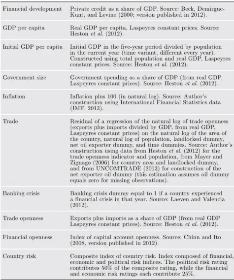
(29) Luisa Blanco | FINANCE, GROWTH, AND INSTITUTIONS IN LATIN AMERICA. 207. obtained from Chinn and Ito’s (2008) database, updated in March 2013, and data on inflation are obtained from the International Financial Statistics (IMF, 2013). Banking crisis data are obtained from Laeven and Valencia (2012). Country risk data are obtained from Political Risk Services Group (2013). Other data used to construct a measure of trade openness that is exogenous in the growth equation come from the United Nations Commodity Trade Statistics Database (UNCOMTRADE, 2013) and Mayer and Zignago (2006). Table A1. Variable description and source Financial development. Private credit as a share of GDP. Source: Beck, DemirgucKunt, and Levine (2000; version published in 2012).. GDP per capita. Real GDP per capita, Laspeyres constant prices. Source: Heston et al. (2012).. Initial GDP per capita. Initial GDP in the five-year period divided by population in the current year (time variant, dif ferent every year). Constructed using total population and real GDP, Laspeyres constant prices. Source: Heston et al. (2012).. Government size. Government spending as a share of GDP (from real GDP, Laspeyres constant prices). Source: Heston et al. (2012).. Inflation. Inflation plus 100 (in natural log). Source: Author’s construction using International Financial Statistics data (IMF, 2013).. Trade. Residual of a regression of the natural log of trade openness (exports plus imports divided by GDP, from real GDP, Laspeyres constant prices) on the natural log of the area of the country, natural log of population, landlocked dummy, net oil exporter dummy, and time dummies. Source: Author’s construction using data from Heston et al. (2012) for the trade openness indicator and population, from Mayer and Zignago (2006) for country area and landlocked dummy, and from UNCOMTRADE (2013) for construction of the net exporter oil dummy (this estimation assumes oil dummy equals zero for missing observations).. Banking crisis. Banking crisis dummy equal to 1 if a country experienced a financial crisis in that year. Source: Laeven and Valencia (2012).. Trade openness. Exports plus imports as a share of GDP (from real GDP Laspeyres constant prices). Source: Heston et al. (2012).. Financial openness. Index of capital account openness. Source: Chinn and Ito (2008, version published in 2012).. Country risk. Composite index of country risk. Index composed of financial, economic and political risk indices. The political risk rating contributes 50% of the composite rating, while the financial and economic risk ratings each contribute 25%..
(30) 208. LATIN AMERICAN JOURNAL OF ECONOMICS | Vol. 50 No. 2 (Nov, 2013), 179–208. Table A1. (continued)a Political risk. Contains the following 12 components: government stability, socioeconomic conditions, investment profile, internal conflict, external conflict, corruption, military in politics, religious tensions, law and order, ethnic tensions, democratic accountability, and bureaucracy quality.. Financial risk. Composed of the following 5 components: foreign debt as a percentage of GDP, foreign debt service as a percentage of exports of goods and services, current account as a percentage of exports of goods and service, net international liquidity as months of import cover, and exchange rate stability.. Economic risk. Composed of the following 5 components: GDP per capita, real GDP growth, annual inflation rate, budget balance as a percentage of GDP, current account as a percentage of GDP.. Government stability. This indicator relates to the government’s ability to carry out its declared programs and its ability to stay in of fice. This indicator is composed of government unity, legislative strength and popular support.. Investment profile. This indicator is related to risks to investment, and is composed of contract viability/expropriation, profits repatriation, and payment delays.. Internal conflict. Indicator related to internal political violence and its actual or potential impact on governance. It is composed of civil war/coup threat, terrorism/political violence, and civil disorder.. Socioeconomic conditions. Constructed using data on unemployment, consumer confidence and poverty to measure socioeconomic pressures at work and in society that can lead to social dissatisfaction.. Foreign debt. Index based on foreign debt as a percentage of GDP.. *The source for variables in this section is Political Risk Services (2013)..
(31)
Figure

+3
Documento similar
The average growth of Latin America contrasts with that of Mexico, where the growth of the gross domestic product (GDP) in 1994–2015 was 2.5 percent (ECLAC, 2016: 16) The growth
Few firms have foreign affiliates outside South America: two in the United States, two in Europe and three in Latin American investment-entrepôt countries.. Our findings
GOVERNANCE AND FOREIGN DIRECT INVESTMENT IN LATIN AMERICA: A PANEL GRAVITY MODEL APPROACH* Turan Subasat** Sotirios Bellos*** It is widely argued that good governance is an
One of the main lines of research where regional and urban economics should deepen in Latin America is the relationship between concentration and growth and particularly the
NATURAL DISASTERS AND POVERTY IN LATIN AMERICA: WELFARE IMPACTS AND SOCIAL PROTECTION SOLUTIONS Alejandro de la Fuente* The World Bank [email protected].. atin
4 REMEF The Mexican Journal of Economics and Finance COVID-19 Pandemic Initial Effects on the Idiosyncratic Risk in Latin America This work aims to estimate the idiosyncratic risk
Notes for Equality N°17 July 2015 Femicide or feminicide as a specific type of crime in national legislations in Latin America: an on-going process By 2015 16 countries in Latin
CHINA´S FINANCING IN THE WORLD: THEORY, INSTITUTIONS, AND INTERNATIONAL CASE STUDIES 01 FOREIGN FINANCIAL FLOWS AND THE BALANCE OF PAYMENTS 21 CONSTRAINT ON LATIN AMERICA´S GROWTH
