A population of eruptive variable protostars in VVV
C. Contreras Pe˜na,
1,2,3‹P. W. Lucas,
2‹D. Minniti,
1,4R. Kurtev,
5,3W. Stimson,
2C. Navarro Molina,
3,5J. Borissova,
5,3M. S. N. Kumar,
2,6M. A. Thompson,
2T. Gledhill,
2R. Terzi,
2D. Froebrich
7and A. Caratti o Garatti
81Departamento de Ciencias Fisicas, Universidad Andres Bello, Republica 220, Santiago, Chile 2Centre for Astrophysics Research, University of Hertfordshire, Hatfield AL10 9AB, UK
3Millennium Institute of Astrophysics, Av. Vicuna Mackenna 4860, 782-0436, Macul, Santiago, Chile 4Vatican Observatory, V-00120 Vatican City State, Italy
5Instituto de F´ısica y Astronom´ıa, Universidad de Valpara´ıso, ave. Gran Breta˜na, 1111, Casilla 5030, Valpara´ıso, Chile 6Instituto de Astrofisica e Ciencias do Espaco, Universidade do Porto, CAUP, Rua das Estrelas, P-4150-762 Porto, Portugal 7Centre for Astrophysics and Planetary Science, University of Kent, Canterbury CT2 7NH, UK
8Dublin Institute for Advanced Studies, School of Cosmic Physics, Astronomy and Astrophysics Section, 31 Fitzwilliam Place, Dublin 2, Ireland
Accepted 2016 October 28. Received 2016 October 28; in original form 2016 February 16
A B S T R A C T
We present the discovery of 816 high-amplitude infrared variable stars (Ks >1 mag) in
119 deg2of the Galactic mid-plane covered by the VISTA Variables in the Via Lactea (VVV)
survey. Almost all are new discoveries and about 50 per cent are young stellar objects (YSOs). This provides further evidence that YSOs are the commonest high-amplitude infrared variable stars in the Galactic plane. In the 2010–2014 time series of likely YSOs, we find that the amplitude of variability increases towards younger evolutionary classes (class I and flat-spectrum sources) except on short time-scales (<25 d) where this trend is reversed. Dividing the likely YSOs by light-curve morphology, we find 106 with eruptive light curves, 45 dippers, 39 faders, 24 eclipsing binaries, 65 long-term periodic variables (P>100 d) and 162 short-term variables. Eruptive YSOs and faders tend to have the highest amplitudes and eruptive systems have the reddest spectral energy distribution (SEDs). Follow-up spectroscopy in a companion paper verifies high accretion rates in the eruptive systems. Variable extinction is disfavoured by the two epochs of colour data. These discoveries increase the number of eruptive variable YSOs by a factor of at least 5, most being at earlier stages of evolution than the known FUor and EXor types. We find that eruptive variability is at least an order of magnitude more common in class I YSOs than class II YSOs. Typical outburst durations are 1–4 yr, between those of EXors and FUors. They occur in 3–6 per cent of class I YSOs over a 4 yr time span.
Key words: stars: AGB and post-AGB – stars: low-mass – stars: pre-main-sequence – stars: protostars – stars: variables: T Tauri, Herbig Ae/Be – infrared: stars.
1 I N T R O D U C T I O N
The VISTA Variables in the Via Lactea (VVV; Minniti et al.2010)
survey has mapped a 560 deg2area containing ∼3×10⁸ point
sources with multi-epoch near-infrared (IR) photometry. The sur-veyed area includes the Milky Way bulge and an adjacent section of the mid-plane. The survey has already produced a deep near-IR
Atlas in five bandpasses (Z,Y,J,H,Ks) and the final product will
include a second epoch of the multifilter data and a catalogue of
more than 106variable sources.
E-mail:[email protected](CCP);[email protected](PWL)
One of the main scientific goals expected to arise from the fi-nal product of VVV is the finding of rare variable sources such as Cataclysmic Variables and RS CVn stars, among others (see Catelan
et al.2013, for a discussion on classes of near-IR variable stars that
are being studied with VVV). One of the most important outcomes is the possibility of finding eruptive variable young stellar objects (YSOs) undergoing unstable accretion. Such objects are usually assigned to one of two subclasses: FUors, named after FU Orio-nis, have long duration outbursts (from tens to hundreds of years); EXors, named for EX Lupi, have outbursts of much shorter duration (from few weeks to several months). Both categories were optically defined in the first instance and fewer than 20 are known in total
shorter periods of unstable accretion at a much higher rate. If this is true, it might explain both the observed under-luminosity of low-mass, class I YSOs (the ‘Luminosity problem’; see e.g. Kenyon
et al.1990; Evans et al.2009; Caratti o Garatti et al.2012) and
the wide scatter seen in the Hertzsprung–Russell diagrams of
pre-main-sequence (PMS) clusters (Baraffe, Chabrier & Gallardo2009;
Baraffe, Vorobyov & Chabrier2012).
In the search for this rare class of eruptive variable stars, Contreras
Pe˜na et al. (2014) studied near-IR high-amplitude variability in the
Galactic plane using the two epochs of UKIDSS Galactic Plane
Sur-vey (UGPS)K-band data (Lawrence et al.2007; Lucas et al.2008).
Contreras Pe˜na et al. found that ∼66 per cent of high-amplitude
variable stars selected from UGPS data releases DR5 and DR7 are located in star-forming regions (SFRs) and have characteristics of YSOs. They concluded that YSOs likely dominate the Galactic disc population of high-amplitude variable stars in the near-IR. Spec-troscopic follow-up confirmed four new additions to the eruptive variable class. These objects showed a mixture of the characteris-tics of the optically defined EXor and FUor subclasses. Two of them
were deeply embedded sources with very steep 1–5μm spectral
en-ergy distributions (SEDs), though showing ‘flat-spectrum’ SEDs at longer wavelengths. Such deeply embedded eruptive variables are regarded as a potentially distinct additional subclass, though only a few had been detected previously: OO Ser, V2775 Ori, HOPS
383 and GM Cha (see Hodapp et al. 1996; K´osp´al et al.2007;
Persi et al.2007; Caratti o Garatti et al.2011; Safron et al.2015).
With the aims of determining the incidence of eruptive variability among YSOs and characterizing the phenomenon, we have under-taken a search of the multi-epoch VVV data set. In contrast to UGPS, the ongoing VVV survey offers several dozen epochs of
Ks data over a time baseline of a few years. We expect that the
VVV survey will also be used to identify YSOs by the common low-amplitude variability seen in nearly all such objects (e.g. Rice,
Wolk & Aspin2012). This will complement studies in nearby star
formation regions and in external galaxies, such as theSpitzer
YSO-VAR programme (e.g. Wolk et al. 2015) and a two-epoch study
of the Large Magellanic Cloud with Spitzer SAGE survey data
(Vijh et al.2009).
We have divided the results of this work in two publications. In this first study, we present the method of the search and a general discussion on the photometric characteristics of the whole sample of high-amplitude variables in the near-IR. We present the follow-up and spectroscopic characteristics of a large subsample of candidate eruptive variable stars in a companion publication (Contreras Pe˜na
et al.2016, hereafterPaper II).
In Section 2 of this work, we describe the VVV survey, the data and the method used to select high-amplitude IR variables. Section 3 describes the make up and general properties of the sample, the
of our results.
2 V V V
The regions covered by the VVV survey comprise the bulge region
within−10◦<l<+10◦and−10◦<b<+5◦and the disc region in
295◦<l<350◦and−2◦<b<+2◦(see e.g. Minniti et al.2010).
The data are collected by the Visible and Infrared Survey Tele-scope for Astronomy (VISTA). The 4 m teleTele-scope is located at Cerro Paranal Observatory in Chile and is equipped with a
near-IR camera (Vnear-IRCAM) consisting of an array of 16 2048×2048
pixels detectors, with a typical pixel scale of 0.339 arcsec, with
each detector covering 694×694 arcsec2. The detectors are set
in a 4×4 array and have large spacing along thex-andy-axis.
Therefore, a single pointing, called a ‘pawprint’, covers 0◦.59 giving
partial coverage of a particular field of view. A continuous coverage of a particular field is achieved by combining six single point-ing with appropriate offsets. This combined image is called a tile. The VVV survey uses the five broad-band filters available in
VIR-CAM,Z(λeff=0.87μm), Y(λeff=1.02μm),J(λeff=1.25μm),
H(λeff=1.64μm) andKs(λeff=2.14μm).
The VVV survey area is comprised of 348 tiles, 196 in the bulge and 152 in the disc area. Each tile was observed in a single
near-contemporaneous multi-filter (ZYJHKs) epoch at the beginning of
the campaign, with an exposure time of 80 s per filter. A second
epoch of contemporaneousJHKswas observed in 2015. The
vari-ability monitoring was performed only inKswith an exposure time
of 16 s.
The images are combined and processed at the Cambridge As-tronomical Survey Unit (CASU). The tile catalogues are produced from the image resulting from combining six pawprints. The cat-alogues provide parameters such as positions and fluxes from dif-ferent aperture sizes. A flag indicating the most probable
morpho-logical classification is also provided, with ‘−1’ indicating stellar
sources, ‘−2’ borderline stellar, ‘1’ non-stellar, ‘0’ noise, ‘−7’
indicating sources containing bad pixels and finally class= −9
re-lated to saturation (for more details on all of the above, see Saito
et al.2012).
Quality control (QC) grades are also given by the European Southern Observatory (ESO) according to requirements provided
by the observer. The constraints for VVVKsvariability data are:
seeing<2 arcsec, sky transparency defined as ‘thin cirrus’ or better.
The ‘master epoch’ of multifilter data taken for each tile in a
con-temporaneousJHKsobserving block and a separateZYobserving
block have more stringent constraints: seeing<1.0, 1.0, 0.9, 0.9,
0.8 inZ,Y,J,H,Ks, respectively, and sky transparency of ‘clear’
(QC A), almost satisfied where, for example, some of the
param-eters are outside the specified constraints by<10 per cent (QC B)
and finally not satisfied (QC C).
2.1 Selection method
In order to search for variable stars, we used the multi-epoch data base of VVV comprising the observations of disc tiles with
|b| ≤1◦taken between 2010 and 2012. We added the 2013–20151
data later to assist our analysis but they were not used in the se-lection. The catalogues were requested and downloaded from the CASU. We used catalogues of observations with QC grades A, B or C. Catalogues with QC grades C are still considered in order to increase the number of epochs. Some of them were still useful for our purposes. However, a small number of catalogues still presented some issues (e.g. zero-point errors, bad seeing) making them use-less and as such were eliminated from the analysis. The number of catalogues in each tile varied from 14 to 23 epochs, with a median of 17 epochs per tile. When the 2013–2015 data were added, the number of epochs available for the light curves rose to between 44
and 59.Ksphotometry is derived fromapermag3aperture fluxes
(2 arcsec diameter aperture).
For each tile, the individual catalogues are merged into a single master catalogue. The first catalogue to be used as a reference was selected as the catalogue with the highest number of sources on it.
In every case, this corresponded to the catalogue from the deepKs
observation (80 s on source), which was taken contemporaneously
with theJ- andH-band data (in 2010). For all other epochs, the time
on source was 16 s.
Fig.1shows the typical scatter shown by stars at different
mag-nitudes across the analysed range. Here we can see considerable scatter at bright magnitudes, due to effects of saturation and the faint end of the distribution, which is dominated by photon noise. High-amplitude variable star candidates are selected from the mas-ter catalogue from stars which fulfilled the following crimas-teria in the 2010–2012 data:
(i) Detection with a stellar morphological classification (class=
−1) in every available epoch.
(ii) Ellipticity with ell<0.3 in every epoch.
(iii) The absolute difference (Ks) between the brightest (Ks,max)
and faintest point (Ks,min) in the light curve of the source to be larger
than 1 mag (similar to the analysis in Contreras Pe˜na et al.2014).
The requirement for a detection at every available epoch in the 2010–2012 interval was designed to exclude most transient objects such as novae, as well as reducing the number of false positives. This was the initial classification scheme. However, we observed that for each tile we were selecting a large number of sources as variable
star candidates. Fig.2shows the averageKsmagnitude versusKs
for variable stars in one of the VVV tiles. The figure shows that the majority of stars selected in the original classification scheme are located at the bright and faint ends of the distribution. The latter arise due to unreliable photometry at this faintest part. The VISTA detectors also become increasingly non-linear when reaching the saturation level. This non-linearity is corrected for in the creation
1We included a singleK
sdata point from 2015 observations, corresponding
to the epoch with contemporaneousJHKsphotometry. Note that our analysis
of the light-curve morphologies and periods is based on the 2010–2014 data only (Section 4.1). The 2015 data became available only after that was complete but they were used in the colour variability analysis (see Section 4.2).
Figure 1. 2010–2012 light curves of ‘non-variable’ VVV objects (i.e. not classified as high-amplitude variables in our analysis). These are presented to show the typical scatter in magnitude across the analysed magnitude range. We note that photometry for the brightest star is the standard CASU pipeline photometry.
of the catalogues, but differences between the magnitudes of the same object can still be observed, even for objects classified as
stellar sources (Saito et al.2012). Fig.10 in Saito et al. (2012)
shows that when comparing theKsmagnitudes of stellar sources
found in overlapping regions of adjacent disc tiles, stars found at the brighter end show an increasing difference in magnitude (an effect
also observed in Cioni et al.2011; Gonzalez et al.2011). This effect
would explain the large differences observed at the brighter end of
Fig.2. This part of the distribution also shows marked ‘finger-like’
sequences. Each of the sequences can be explained by the fact that the VISTA detectors have different saturation levels. In order to minimize these effects, we applied an additional cut.
(iv) We separated the averageKsdistribution of Fig.2into bins of
0.5 mag and derived the mean and standard deviation,σ, onKsfor
each bin. In order to select an object as a candidate variable star, we
required itsKsto be 3σabove the meanKsat the corresponding
magnitude level. This 3σ line is shown in red in Fig.2where we
can see that it is able to account for the non-linearity effects at the bright end of the distribution.
This additional constraint reduced the number of variable star candidates by a large factor. The initial requirements yield 158 478 stars; the additional cut reduced this to 5085 stars. After the
catalogue-based selection, we constructed 1 arcmin ×1 arcmin
cut-out images around each candidate for every available epoch. Variable stars were confirmed as real through visual inspection of
the individual images (an example is shown in Fig.3). In some cases,
we performed manual photometry withIRAFin order to confirm the
Figure 2. KsversusKsfor one of the VVV tiles studied in this work, showing stars with class=−1 and ellipticity<0.3 in every epoch (black circles).
Variable star candidates which fulfil the conditionKs>1 mag are shown as blue circles. The red solid line marks the additional 3σcut applied to the objects
as explained in the text. Stars above this line are selected for subsequent visual inspection.
Figure 3. Example of the images used to visually inspect variable star candidates. In this case, we show the images, taken between 2010 and 2012, of variable star VVVv322. Each image has a size of 1 arcmin×1 arcmin. The star gets brighter towards the end of the sequence.
sources, diffraction spikes and stars that were found on the edge of tiles. In the case of saturation, if this effect was present, it was quite evident in individual images. In most cases, saturation was observed in every single epoch, thus the variability observed in the light curve plots was not real and the source was marked as such.
This selection method yielded a total of 840 real variable stars. However, 25 of them are found twice as they are covered by adjacent tiles in VVV. The final list of VVV high-amplitude IR variables consists of 816 stars. This includes one variable star, VVVv815, that showed large variability in 2010 but did not meet all the selection criteria. The average magnitude for objects in the selected sample
was found in the range 10.3<Ks<16.9 mag.
Our requirement for a high-quality detection at every epoch be-tween 2010 and 2012 (see items i and ii) is bound to cause us to miss
some real variables, very likely including some of the faintest or
highest amplitude variables if they dropped belowKs∼16 during
that time or if they became saturated and were therefore no longer classified as point sources. A significant fraction of all VVV sources are blended with adjacent stars and they can fail to pass our cuts on the morphological class and ellipticity at one or more epochs in consequence. The same can be true for YSOs with extended
reflection nebulae or strong H2 jets, as they might have slightly
extended morphologies and fail to be classified as point sources
(see e.g. Chen et al.2009; Ward et al.2016). However, sources that
pass these quality cuts are likely to be unblended and therefore to have reliable photometry (photometry from the VISTA pipeline is not always reliable for faint stars in crowded fields, see e.g. Saito
et al.2012). In order to check the reliability of the pipeline
Figure 4. PSF (red triangles) versus aperture photometry (open circles) of star VVVv316. PSF photometry is shown only for data points classified as ‘good’ or ‘good but faint’ byDOPHOT.
point spread function (PSF) fitting photometry of all stars in tile
d069 withDOPHOT(Schechter, Mateo & Saha 1993). The results
confirmed that the variables found by our selection have reliable
pipeline photometry. This is illustrated in Fig.4for variable star
VVVv316, where the comparison ofDOPHOTand VISTA pipeline
photometry shows close agreement.
We investigated the incompleteness of our selection by examining two widely separated VVV disc tiles (d064 and d083), in which we removed our class and ellipticity cuts and required a minimum of only one detection in each year from 2010 to 2012 (with a stellar profile classification). This continues to select against transients and perhaps the most extreme variable YSOs but it allows us to assess incompleteness due to blending, which can cause sources to be absent or to have different profile classifications at different epochs. We found that this more relaxed selection added over 400 additional
candidates in the two tiles down to (mean)Ks=15.5, an increase
of more than a factor of 10. Following visual inspection, we found that the number of real high-amplitude variables was increased by a
factor of∼2, up to a limit ofKs=15.5. At fainter mean magnitudes
the completeness of our selection with criteria (i)–(iv) falls more steeply because most high-amplitude variables will not satisfy the quality cuts at every epoch as the sensitivity limit is approached.
A case of this selection effect is found in a variable star VVVv815
mentioned above. It showed a large variation (Ks>1 mag) in the
analysis of an early release of 2010 data. However, the star does not show up as a variable star candidate in the analysis described above. Inspection of the master catalogue for the respective tile shows that the star has a classification different from stellar in 3 out of 18 epochs available for tile d090 in the 2010–2012 period. This star is included in our final list of VVV high-amplitude variables because it is also part of the sample that has follow-up spectroscopic observations.
The number of stars in the analysed VVV area that fulfil criteria (i) and (ii) above is 12 789 000 stars. Considering the number of real variable stars, we see that high-amplitude IR variability was observed in approximately 1 out of 15 000 stars in the Galactic
mid-plane at 295◦< l <350◦.
2.2 Issues with saturation
The aforementioned problems of saturation still affect a small num-ber of stars in our sample. This effect can become important when
individual epochs of stars in our sample are brighter thanKs=12
Table 1. Ksphotometry of the 816 high-amplitude variable stars from VVV.
The full version of the table is available online.
ID MJD-55200 Ks Ks,err
mag. Saturation will reduce the flux at the inner core of the star, thus the magnitude of the star derived by using smaller diameter aperture than the default 2 arcsec aperture will be fainter than the magnitude obtained from the default aperture.
In order to check whether the star is saturated, we first ob-tain the magnitudes from aperture photometry using the measure fluxed from five different diameters for the apertures. These di-ameters are 1 (Apermag1), 1.41 (Apermag2), 2 (Apermag3), 2.82 (Apermag4) and 4 arcsec (Apermag5). We find that saturated stars show relatively large differences between the magnitudes from the first three apertures and we set a threshold for saturation as stars
having both Apermag1-Apermag3 > 0.05 mag and
Apermag2-Apermag3>0.02 mag. Thus, any individual epoch of a star with
Apermag3<12 mag (in theKspassband) and having these
differ-ences is flagged as saturated.
In order to correct for saturation, we follow Irwin (2009) and
defined a ring outside the saturated core to obtain a new flux esti-mate. We then determine an aperture correction for the ring from a set of bright, unsaturated stars found within 5 arcmin of our object of interest. In our analysis, we derived new fluxes using the ring defined by Apermag2 and Apermag4. Comparison with 2MASS
Ksphotometry indicates that this choice of apertures extends the
dynamic range by 2.5 mag, relative to the pipeline photometry. We
caution that comparison with 2MASSKsphotometry indicates that
while this approach provides correct magnitudes, the uncertainties are large, typically 0.2 mag.
In Table1, we present the 2010–2015 photometry for the 816
high-amplitude variable stars from VVV.
3 H I G H - A M P L I T U D E I R VA R I A B L E S F R O M V V V
3.1 General characteristics
The selection method of Section 2.1 yields 816 high-amplitude
(Ks>1 mag) IR variables. In order to study the properties of these
stars, we searched for additional information in available public data bases. This search can be summarized as follows.
(i) SIMBAD: we query the SIMBAD data base (Wenger
et al.2000) for astronomical objects within a radius of 5 arcmin
centred on the VVV object.
(ii) Vizier: additional information was provided with the use of
the Vizier data base (Ochsenbein, Bauer & Marcout2000). Here
were visually inspected.
In addition, we used the WISEimage service within IRSA to
inspect multicolour images of the areas around our variable stars, in order to establish a possible association of the VVV object with an SFR.
The general properties of the sample can be found in Table2.
Column 1 presents the original designation given to the sources. Column 2 corresponds to the full VVV designation for the source. Coordinates for the objects are given in Columns 3 and 4, with columns 5 and 6 presenting the Galactic coordinates of the sources.
In columns 7–11, we present the nearly contemporaneousZ,Y,J,
H,Ksphotometry from VVV. Column 12 givesKs, the absolute
value of the peak-to-trough difference from the 2010–2014 light
curves from VVV. Column 13 presentsαclass, the 2–23μm spectral
index parameter that relates to the evolutionary class of sources that appear to be associated with SFRs (the method and data used to estimate this parameter is explained in Section 4.3). In column 14, we present whether the object is likely associated with SFRs or not, whilst column 15 presents the classification of the object from its light curve. The latter is discussed throughout the text. Finally, in column 16, we present the approximate period for variable stars where we are able to measure this parameter.
Most of the variable stars are unknown from searches in SIM-BAD and Vizier (∼98 per cent). Among the known variables, there are two novae, Nova Cen 2005 and Nova Cen 2008 (Hughes
et al.2010; Saito et al.2013), two eclipsing binaries (EBs),
EROS2-GSA J132758-631449 and PT Cen (Derue et al. 2002; Budding
et al.2004), one high-mass X-ray binary, BR Cir (see e.g. Tudose
et al.2008) and nine OH/IR stars. Among the objects not previously
classified as variable stars, 159 are found in theSpitzer/GLIMPSE
catalogue of intrinsically red sources from Robitaille et al. (2008),
with the majority being classified as likely YSOs from their mid-IR colours and brightness.
3.2 YSO population
At this point, the reader should note that most of the variables are
listed as spatially associated with SFRs (∼65 per cent, falling to
∼50 per cent after allowing for chance projection by non-YSOs, see Section 3.3, 3.4 and 4) and these stars have spectral indices that indicate a class I or flat-spectrum evolutionary status, therefore they are likely in an early evolutionary stage. They are usually
sufficiently red to be undetected (i>21 mag) in sensitive panoramic
optical surveys such as VPHAS+(Drew et al.2014) unlike most of
the known FUor and EXors. The spectral indices of the YSOs are discussed later in Section 4.3 following classification of the light curves and an attempt to decontaminate chance projections of other variables in SFRs.
whereAis the area covered by the survey (Bate et al.1998, and
references therein). This correlation function is valid as long as the
separationsθ are smaller than the angular length of the sample.
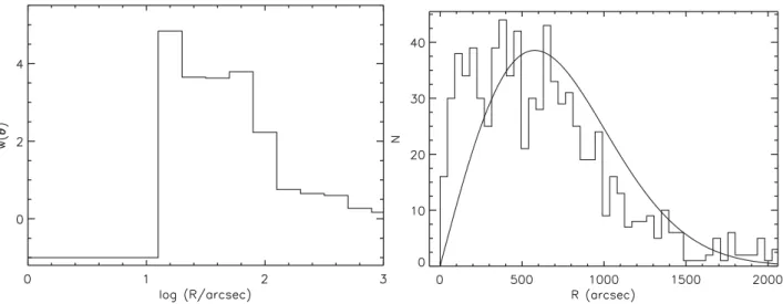
We show the two-point correlation function in Fig.6. We can see
that we do not find any pairs for separationsθ <20 arcsec, hence
w(θ)= −1. For separations between 20 and 100 arcsec,w(θ) is
larger than the values expected for random pairings (w(θ)=0) and
it remains somewhat above zero for separations up to a few hundred
arcseconds. This nearest neighbour distribution of Fig.6also shows
an excess of close neighbours at distancesR<200 arcsec, compared
to the expected number from a random (Poisson) distribution. Thus, we are confident that we are tracing clustering in the VVV sample, on a spatial scale similar to that of distant Galactic clusters and star formation regions.
As an illustration of how variable stars in VVV are preferentially
located in areas of star formation, Fig.7shows theKsimage of the
area covered in tile d065. 25 highly variable stars are found in this tile and it is clear that these are not evenly distributed along the area covered in d065 and instead are found clustered around an area of star formation, which is better appreciated in the cut-out image
fromWISE(Wright et al.2010).
To establish a likely association with an SFR, we used the criteria
established in the UGPS search (see Contreras Pe˜na et al.2014),
which were based on entries in the SIMBAD data base and the Avedisova catalogue within a 5 arcmin radius of each
high-amplitude variable. In addition, we also checkWISEimages for
evidence of star formation in the area of the object, e.g. evidence
of bright extended 12μm emission near the location of the objects
or the finding of several stars with redW1−W2 colours (sources
appearing green, yellow or red inWISEcolour images) around the
VVV object. We find that 530 of our variable stars are spatially associated with SFRs, which represents 65 per cent of the sample, remarkably similar to the observed association in UGPS objects
(Contreras Pe˜na et al.2014).
3.4 Contamination by non-YSOs
In Contreras Pe˜na et al. (2014), we estimated that about 10 per cent
Figure 6. (left) Two-point angular correlation function of the sample of VVV high-amplitude variables. (right) Nearest neighbour distribution for the same sample. The smooth curve represents the expected distribution of a random (Poisson) distribution.
higher extinction in the Galactic mid-plane and the brighter satura-tion limit of VVV than UGPS allows for a larger number of bright evolved variable stars to show up in our results. To determine the percentage of objects that might be catalogued as likely associated with SFRs by chance, we used the following method.
(1) Create a master catalogue of objects in the 76 tiles that were classified as stars in each of the epochs from the 2010–2012 analysis.
(2) Select 816 stars randomly from this catalogue and query SIMBAD for objects found in a 5 arcmin radius.
(3) Count the number of objects within this radius that were classified in any of the categories that could relate to star
forma-tion. This categories included T Tauri and Herbig Ae/Be stars, HII
regions, Dark clouds, dense cores, millimeter and submillimeter sources, FU Orionis stars, among others.
(4) Repeat items (2) through (3) 40 times.
Fig.8shows the number of stars found within 5 arcmin of the
VVV object and that were classified in the categories shown above,
Nsimbadversus the percentage of VVV objects with this number. It
is already apparent that the percentage of chance selection will be higher than that estimated from GPS. However, we note that in order
for an object to be flagged as associated with an SFR in Table2, we
needed at least four SIMBAD objects to appear within the 5 arcmin
radius, thus giving us an estimate that∼30 per cent of the non-YSO
population is spatially associated with an SFR by chance. Inspection
ofWISEimages of 100 randomly selected sources yields a similar
fraction of chance associations but most of these were also identified
as SFR-associated from the SIMBAD results, so theWISEdata only
slightly increased the chance association fraction. The Avedisova catalogue added an even smaller fraction of chance associations
not indicated by the SIMBAD andWISEdata, so the final chance
association probability for non-YSOs with star formation regions is 35 per cent.
The number of non-YSOs in the SFR-associated sample is less than 35 per cent because non-YSOs do not dominate the full high-amplitude sample but constitute about half of it. We found 286/816 (35 per cent) of variables outside SFRs, i.e. in 65 per cent of the area, suggesting that 54 per cent (35/0.65) of the sample is composed of objects other than YSOs but this neglects the fact that some YSOs will be members of SFRs that are not known in the literature nor
visible inWISEimages (see Section 3.5). Consequently, random
addition of 35 per cent of half of the total sample of 816 variables to the SFR-associated sample would be expected to cause only 27 per cent contamination of the SFR-associated subsample by non-YSOs. This conclusion that the SFR-associated population of variables is dominated by bona fide YSOs is supported by the two
colour diagrams (Figs10and22) and light curves of the population
(see Sections 3.5 and 4.1), which differ from those outside SFRs. We note that the results of spectroscopic follow-up of a subsample
of VVV objects associated with SFRs (Paper II) show a figure of
25 per cent, a consistent figure despite some additional selection effects in that subsample.
3.5 Properties of variables outside SFRs
To establish the nature of the objects that could be contaminating our sample of likely YSOs and may also be interesting variable stars, we study the properties of objects found outside areas of star formation. Many of these are listed in SIMBAD as IR sources (from the IRAS and MSX6C catalogues) and associated with OH masers, as well as being catalogued as evolved stars in previous surveys. Visual inspection of their light curves also shows that a large percentage
of objects have periodic variability, with P > 100 d, whilst the
remainder of the sample shows variability over shorter time-scales
of the order ofP<20 d. We use the phase dispersion minimization
(PDM; Stellingwerf1978) algorithm found in theNOAOpackage in
IRAFto search for a period in the light curve of these objects. This
allows us to derive the periods or at least the approximate time-scale of the variability of objects found outside areas of star formation. To
provide a comparison with thePDMresults, we also used theGATSPY
LOMBSCARGLEFASTimplementation of the Lomb–Scargle algorithm,
which benefits from the automatic optimization of the frequency
grid so that significant periods are not missed. We found thatPDM
was generally better for the purpose of this initial investigation. The Lomb–Scargle algorithm is designed to detect sinusoidal variations,
whereasPDMmakes no assumptions about the form of the light curve
and is therefore much more sensitive to the periods of EBs, for example. The Lomb–Scargle method did help with the classification of a small number of long period variables (LPVs).
Figure 7. The top graph shows theKsimage of tile d065 along with the
high-amplitude variable stars found in this region. The clustering of the variable stars is already apparent in this image. The bottom graph shows the WISEfalse colour image of the same region (blue=3.5 µm, green=4.6 µm, red=12µm). Here, the fact that variable stars preferentially locate around areas of star formation can be better appreciated.
X-ray binary), 45 per cent of them are LPVs and 17 per cent are EBs where we are able to measure a period. In addition, 30 per cent of the sample is comprised of objects in which variability seems to occur on short time-scales. The light curves of many objects in the latter group resemble those of EBs with measured periods, but with only one or two dips sampled in the data set. We suspect that most of these could also be EBs but we are not able to establish the periods. Finally, we also find 18 objects (6 per cent) that do not
appear to belong to any of the former classes. In Fig.9, we show two
examples of objects belonging to these different subclasses where a
Figure 8. Percentage of objects flagged as likely associated with SFRs as a function of the number of objects classified in the categories that could relate to star formation found within a 5 arcmin radius query in SIMBAD.
Figure 9. Examples ofKslight curves for objects not associated with SFRs.
(top) the LPV VVVv215. (bottom) The EB VVVv203.
period could be derived. The LPV VVVv215 is typical of many of the dusty Mira variables in the data set that show long-term trends caused by changes in the extinction of the circum-stellar dust shell. These trends are superimposed on the pulsational, approximately
sinusoidal variations, with the result that theKsmagnitude, at a
Figure 10. (top) OverallKs distribution (from 2010 data) of objects not
associated with SFRs (black dashed-dotted line) and the same distribution separated for LPVs (solid blue line), EBs and known objects (solid orange line) and other classes of variable stars (solid red line). (bottom) (J−H), (H−Ks) colour–colour diagram for LPVs (blue circles), EBs and known
objects (orange circles) and other classes of variable stars (red circles). In the diagram, arrows mark lower limits. The solid curve at the lower left indicates the colours of main-sequence stars. The short dashed line is the CTTS locus of Meyer, Calvet & Hillenbrand (1997) and the long dashed lines are the reddening vectors.
The objects belonging to different classes show very different
properties. Fig.10shows theKsdistribution for these objects, where
it can be seen that the LPVs dominate the bright end of the
distri-bution with a peak atKs∼11.8 mag and showing a sharp drop at
brighter magnitudes, probably due to the effects of saturation. EBs and other classes are usually found at fainter magnitudes. The
near-IR colours of the two samples (bottom plot of Fig.10) show that
LPVs tend to be highly reddened objects or have larger (H−Ks)
colours than EBs and other classes, which usually have the colours of lightly reddened main sequence and giant stars. We will see in
Section 4 that this low reddening and lack ofK-band excess (in most
cases) distinguishes the EBs and other shorter period variables from the sample spatially associated with SFRs, so contamination of the SFR sample by these shorter period variables should not be very significant.
The colour–colour diagram of Fig. 10 also supports the idea
that this sample might contain some bona fide YSOs that are not
revealed by our searches of SIMBAD and theWISEimages, as
mentioned in our discussion of contamination. In the figure, we
observe objects (red circles) that show (H−Ks) colour excesses
and are neither known variables nor classified as LPVs or EBs. By simply selecting red circles located to the right of the reddening vector passing through the reddest main-sequence stars, we estimate that 44 objects have colours consistent with a YSO nature. This would represent 15 per cent of objects outside SFRs and 5 per cent of the full sample of 816 variables. A more detailed study would of course be needed to confirm their nature as YSOs. We also note that the lower left part of the classical T Tauri stars (CTTS) locus plotted in the figure extends into the region occupied by lightly reddened main-sequence stars so, in principle, some of these individual red circles can potentially be YSOs.
The bright LPVs are very likely pulsating asymptotic giant branch (AGB) stars. These type of stars are usually divided into Mira
vari-ables, which are characterized by displaying variability ofK>0.4
mag and with periods in the range 100< P< 400 d and
dust-enshrouded AGB stars, which are heavily obscured in the optical due to the thick circum-stellar envelopes (CSE) developed by heavy
mass-loss (∼10−4M
yr−1). The latter group, comprised of
carbon-rich and oxygen-carbon-rich stars (the latter often referred to as OH/IR stars
if they display OH maser emission), show larger amplitudes in theK
band (up to 4 mag) and have periods in the range 400<P<2000 d
(for the above, see e.g. Jim´enez-Esteban et al.2006b; Whitelock,
Feast & van Leeuwen2008).
AGB stars are bright objects and should be saturated at the mag-nitudes covered in VVV. However, due to the large extinctions towards the Galactic mid-plane, we are more likely to observe these type of objects in VVV compared to our previous UKIDSS study. We can estimate the apparent magnitude of Mira variables at the different Galactic longitudes covered in VVV and by assuming that
these objects are located at the Galactic disc edge (RGC=14 kpc;
Minniti et al.2011) and then considering other Galactocentric radii.
At a given longitude,l, we derive AV as the mean value of the
interstellar extinction found at latitudes bbetween −1◦ and 1◦.
The interstellar extinction is taken from the Schlegel, Finkbeiner &
Davis (1998) reddening maps and corrected following Schlafly &
Finkbeiner (2011), i.e.E(B−V)=0.86E(B−V)Schlegel. We then
assume that extinction increases linearly with distance, at a rate
AV/Dedge(mag kpc−1), withDedgethe distance to the Galactic disc
edge at the correspondingl. We finally take the absolute magnitude
asMK= −7.25 (Whitelock et al.2008).
Fig.11shows the estimated apparent magnitudes of Mira
vari-ables at differentland at varyingRGC. In the figure, we also show
the magnitude,Ks =11.5, that marks the drop in the number of
the detection of these objects, as observed in the histograms of the
Ksdistribution (Fig.10). We can see as we move away from the
Galactic Centre, a Mira variable would most likely saturate in VVV,
especially atl<310◦. This occurs due to the effects of having
rel-atively larger extinctions towards the Galactic Centre (see bottom
plot of Fig.11) and that a star atRGC=14 kpc is located farther
away from the observer aslapproachesl=0◦. We note that Ishihara
et al. (2011) finds that most AGB stars are found atRGC<10 kpc,
so if we place a Mira variable at smaller Galactic radii (RGC=7,
10 kpc), we see that it is less likely for such a star to show up in our sample. However, variable dust-enshrouded AGB stars, which undergo heavy mass-loss, suffer heavy extinction due to their thick CSE and thus are fainter than Mira variables (AGB stars with
op-tically thick envelopes are found to be∼5Ksmagnitudes fainter
than objects with optically thin envelopes in the work of
Jim´enez-Esteban et al.2006a) and thus less likely to saturate in VVV, even at
Figure 11. (top) ApparentKsmagnitude, derived as explained in the text,
for a Mira variable located at the Galactic disc edge (solid red line). The same value is shown for a Mira located at lower Galactic radiiRGC=10 (blue
line) and 7 kpc (black line). The magnitude where the number of detections for LPVs drops (Ks=11.5 mag) is marked by a dotted line. (bottom)K-band
Galactic extinction column as a function of Galactic longitude.
The observations confirm the trend expected from the analysis
above. Fig.12shows that the number of LPVs increases as we come
closer to the Galactic Centre. In addition, when taking into account AGB stars with measured periods, we confirm that the majority of AGB stars show periods longer than 400 d and large amplitudes (see
lower panel in Fig.12), as expected in heavily obscured AGB stars.
It is interesting to see in the same figure that variable objects with periods longer than 1500 d show lower amplitudes than expected for their long periods. This is similar to the observed trend in the
variable OH/IR stars of Jim´enez-Esteban et al. (2006b). According
to the authors, these objects correspond to stars at the end of the AGB. We note that the apparent lack of high-amplitude objects at longer periods could relate to the fact that more luminous (longer period) objects have smaller amplitudes expressed in magnitudes
(red supergiants often display K< 1 mag; see e.g. van Loon
et al.2008).
This population of bright pulsating AGB stars can also explain
the observed bimodality of theKsdistribution for the full sample of
VVV high-amplitude variable stars (see Fig.13). The peaks of the
distribution occur atKs∼11.8 and 15.8. The peak at the bright end
is at the same magnitude as the peak for LPVs.
When we only plot objects which are found to be likely associated with areas of star formation, the peak at the bright end becomes
less evident (see blue histogram in Fig.13). When we plot only
SFR-associated sources that do not have LPV-like light curves (see Section 4.1) the bimodality almost disappears, as shown by the red
histogram in Fig.13. AGB stars are probably the main source of
contamination in our search for eruptive YSOs in SFRs, especially dust-enshrouded AGB stars which can have IR colours resembling those of YSOs. Hence, it is fortunate that we can remove most of this contamination by selecting against LPV-like light curves.
Figure 12. (top) Overall Galactic longitude distribution of objects outside SFRs (black dashed-dotted line). We also show the same distribution divided into LPVs (blue line), EBs and known objects (orange line) and other classes of variable stars (red line). (bottom) Period versusKsamplitude for LPVs
with a measured period.
Figure 13. Ksdistribution (from 2010 data) of the 816 VVV selected
3.6 YSO source density
Our finding in Section 3.3 that YSOs constitute about half of the detected population of high-amplitude variables in VVV disc fields indicates that they represent the largest single population of high-amplitude IR variables in the Galactic mid-plane, at least in the
range 11< K< 17. We note that extragalactic studies of
high-amplitude stellar variables are dominated by the more luminous
AGB star population (see e.g. Javadi et al. 2015). Our analysis
only considered the VVV disc tiles with|b|<1◦, this amounts to
76 tiles, covering each 1.636 deg2of the sky. After allowing for
the small overlaps between adjacent tiles, the total area covered
in this part of the survey is 119.21 deg2. Adopting a 50 per cent
YSO fraction for the full sample of 816 variables implies a source
density of 3.4 deg−2. As noted in Section 2.1, the stringent data
quality cuts in our selection procedure excluded∼50 per cent of
high-amplitude variables down toKs= 15.5 and a high fraction
at fainter magnitudes where completeness falls (see Fig.13). The
corrected source density is therefore∼7 deg−2.
When considering the source density of high-amplitude IR
vari-ables in the UGPS, Contreras Pe˜na et al. (2014) argued that the
observed source density underestimates the actual source density
due to three main effects: (1) with only two epochs ofK-band data,
most high-amplitude variables will be missed; (2) the source density
rises towards the magnitude cut ofK<16, indicating that many
low-luminosity PMS variables, which are detected at distances of 1.4–2 kpc, would be missed at larger distances and (3) the data set used in the UGPS search of Contreras Pe˜na et al. excludes the mid-plane and is therefore strongly biased against SFRs. The UGPS YSO
source density is estimated to reach 12.7 deg−2when correcting for
these three factors. In the case of VVV, given the higher number of epochs obtained from this survey and that this analysis is not biased against areas of star formation, the source density is only likely to
be affected by item (2) of the UGPS analysis. Fig.13shows the
magnitude distribution of the VVV variables associated with SFRs, where we can see a similar behaviour to the UGPS results, with the density of sources rising steeply towards faint magnitudes. Contrary to the UGPS search, we do not have a hard magnitude cut in the
VVV sample, which includes sources as faint asKs∼17. However,
the number of sources decreases atKs >16, so we estimate an
effective magnitude detection limit ofKs=16.25 mag. This
im-plies that if typical sources from VVV have similar characteristics
to UGPS objects in Cygnus and Serpens (K=14.8,d=1.4–2 kpc),
then we would not detect them at distances d> 3.32 kpc. The
complete sample of star-forming complexes from Russeil (2003)
shows that 83 per cent of them are located beyond these distances. Correcting for this factor, we then estimate a true source density of
41 deg−2, though this figure does not include YSOs with low mass
and luminosity that are too faint to be sampled by VVV due to the
absence of nearby SFRs in the survey area. This figure of 41 deg−2
is three times larger than the one estimated from the UGPS analysis
of Contreras Pe˜na et al. (2014) (12.7 deg−2).
Two effects can account for the larger source density in VVV than UGPS. (1) High-luminosity YSOs are less common, but they can be observed at larger distances. The UGPS study would not find such objects at large distances because the available data set did not cover the mid-plane of the Galactic disc, in which all dis-tant SFRs are located due to their small scaleheight. Since VVV does cover the mid-plane, we are able to detect these rare higher luminosity YSOs. This seems to be supported by the slightly larger distances established for members of the spectroscopic subsample inPaper II. (2) In the UGPS study, most (23/29) of the variables in SFRs were located in just two large SFRs: the Serpens OB2
association and portions of Cygnus X. The much smaller size of the UGPS sample (in number of SFRs and number of variables) meant that there was considerable statistical uncertainty in the area-averaged source density. Moreover, the incidence of high-amplitude variability is greater at the earlier stages of YSO evolution (see Sec-tion 4.3), so the numbers in the UGPS study may have been reduced by a relative lack of YSOs at these stages in the two large SFRs surveyed.
The estimated highly variable YSO source density remains much larger than that estimated for Mira variables in Contreras Pe˜na et al.
(2014), indicating a higher average space density for the variable
YSOs. The observed variables in SFRs also outnumber the EBs and unclassified variables in the magnitude range of this study. However, we are likely to miss a large part of the population of high-amplitude EBs due to the sparse time sampling of VVV.
In Appendix A, we attempt to calculate the source density and space density of high-amplitude EBs from the OGLE-III Galactic
disc sample of Pietrukowicz et al. (2013). In this, we are aided
by a recent analysis of the physical properties of the large sample ofKeplerEBs (Armstrong et al.2014), which indicates that EBs
with high amplitudes in the VVVKsand OGLEIpassbands are
dominated by systems with F- to G-type primaries. We use simple calculations to show that while EBs can have very high amplitudes at optical wavelengths, the eclipse depth should not exceed 1.6 mag
inKs. Similarly, we find that eclipse depths should not exceed 3 mag
inI. These results are supported by the VVV and OGLE-III data sets
(Pietrukowicz et al.2013) in which the distribution of EB amplitudes
falls to zero by these limits. YSOs withKs>1.6 mag are very
numerous in our sample so we conclude that high-amplitude YSOs
greatly outnumber EBs above this limit. BelowKs=1.6 mag, it
is harder to reach a firm conclusion (see Appendix A). The space densities of EBs and those YSOs massive enough to be sampled by
VVV may be comparable at 1< Ks<1.6 mag. High-amplitude
YSOs are likely to be more numerous if the variability extends down to the peak of the initial mass function at low masses, given that high-amplitude EB systems contain a giant with mass of order
1 M.
4 A N A LY S I S O F VA R I A B L E S I N S TA R F O R M AT I O N R E G I O N S
The results presented here concern YSO variability in theKs
band-pass. At these wavelengths, variability in typical YSOs is produced by physical mechanisms (or a combination of them) affecting the stellar photosphere, the star–disc interface, the inner edge of the dust
disc as well as spatial scales beyond 1 au (see e.g. Rice et al.2015).
These mechanisms include cold or hot spots on the stellar
photo-sphere (e.g. Scholz2012), changes in disc parameters such as the
location of the inner disc boundary, variable disc inclination and
changes in the accretion rate (as shown by Meyer et al.1997).
Vari-able extinction along the line of sight can also be responsible for the observed changes in the brightness of YSOs. Dust clumps that screen the stellar light have been invoked to explain the variability observed in Herbig Ae/Be stars and early-type CTTS (group also
known as UX Ori stars; see e.g. Herbst & Shevchenko1999; Eiroa
et al.2002). In other scenarios, variable extinction can be produced
by a warped inner disc dust that is being uplifted at larger radii by a centrifugally driven wind, azimuthal disc asymmetry produced by the interaction of a planetary mass companion embedded within the disc or by occultations in a binary system with a circum-binary
tion depends on the temperature of the spot and the percentage of the photosphere that is covered by such spots, thus sufficiently hot spots can produce larger changes in the magnitude of the system.
The range inKfrom variable extinction is effectively limitless
as it depends on the amount of dust that obscures the star. Large
changes (K>1 mag) have been observed from variable extinction
in YSOs, e.g. AA Tau, V582 Mon (Bouvier et al.2013; Windemuth
& Herbst2014). Nevertheless, variable extinction can be inferred
from colour variability (see e.g. Section 4.2). Wolk et al. (2013)
also estimate that a change in the accretion rate of a class II object
of log ˙M(Myr−1) from−8.5 to−7 yieldsK∼0.75 mag. Thus,
larger changes as observed in eruptive variables will produce large amplitudes.
Given all of the above, it is reasonable to expect variability in our YSO sample to be dominated by accretion-related variability and/or events of obscuration by circum-stellar dust.
4.1 Light-curve morphologies
We have visually inspected the light curves of our 530 SFR-associated variables in order to gain insight into the physical
mech-anism causing the brightness variations. In addition, we usedPDM
inIRAFandLOMBSCARGLEFASTinGATSPYto search for periodicity in
the light curves of our objects. We stress that this is a simple and preliminary classification that is highly influenced by the sparse sampling of VVV. A more detailed study is planned in future, with improved precision by applying the differential photometry method
of Huckvale, Kerins & Sale (2014) to the VVV images. We have
divided the morphologies in the following classifications.
(i) Long-term periodic variables: defined as objects showing
peri-odic variability withP>100 d. This limit is adopted for consistency
with the limit used in the analysis of objects outside of SFRs, with the benefit that contamination by long-period AGB stars will be con-fined to this group. We measure periods for most of these objects, albeit with some difficulty in phase-folding the data in many of them. In this subsample, we find 154 stars, representing 29 per cent of ob-jects spatially associated with SFRs. In Section 3.4, we contended that field high-amplitude IR variables with periodic light curves
(P>100 d) are very likely dust-enshrouded AGB stars, these being
identifiable by their smooth, approximately sinusoidal light curves.
We estimated that∼27 per cent of the 530 SFR-associated variables
would be non-YSOs and up to 45 per cent of these would be LPVs,
implying that this subsample may contain∼64 dusty Mira variables.
Visual inspection of the 154 light curves indicates that while some have a smooth sinusoidal morphology (after allowing for long-term trends due to variable extinction in the expanding circum-stellar dust shell), others display short time-scale scatter superimposed on
there is a larger number of ‘long-term’ periodic variables found
with periods, 100<P<350 d. The 65 blue points are the objects
with short time-scale scatter and the red points are the remaining 89, categorized by careful inspection of the light curves of the 154 long-term periodic variables in SFRs. The blue points clearly
dominate the group withP<350 d and they also have a distinctly
fainter distribution ofKsmagnitudes, similar to that shown in the
red histogram in Fig. 13, which represents all objects in SFRs
except those with Mira-like light curves. As expected, the red points
with Mira-like light curves typically haveKs∼12, similar to the
LPV distribution plotted in Fig.10. We conclude that inspection of
the light curves can separate the evolved star population of LPVs from the YSOs in SFRs with fair success, though we caution that this is an imperfect and somewhat subjective process that can be influenced by outlying data points and our limited knowledge of the time domain behaviour of circum-stellar extinction in dusty Mira systems. The limitations are demonstrated by the presence of a
number of blue points withKs∼12 andP>350 d in the lower panel
of Fig.15and a hint of bimodality even in the ‘decontaminated’
magnitude distribution in Fig.13(red histogram). In the subsequent
discussion of YSOs from our sample, we only include the 65 objects with short time-scale scatter (called LPV-yso) and assume that the other 89 sources are dusty AGB stars or other types of evolved star (or LPV-Mira).
This decontamination of AGB stars reduces the SFR-associated sample to 441 objects. The long-term periodic YSOs represent 15 per cent of this sample.
Periods,P>15 d, are longer than the stellar rotation period of
YSOs or the orbital period of their inner discs (Rice et al.2015).
Some YSOs have been observed to show variability with periods
longer than even 100 d. WL 4 inρOph shows periodic variability
withP=130.87 d (Plavchan et al.2008), which can be explained
by obscuration of the components of a binary system by a
circum-binary disc. TheK-band amplitude of the variability in that system
is somewhat less than 1 mag. However, it is possible to think that a similar mechanism might be responsible for the variations in some
of our objects. Hodapp et al. (2012) show that variable star V371
Ser, a class I object driving an H2 outflow, has a periodic light
curve withP=543 d. The authors suggest that variability arises
from variable accretion modulated by a binary companion. In view of this, the variability in some of the long-term periodic variables
might be driven by accretion and we discuss this inPaper II, based
on spectroscopic evidence for a subsample of them.
(ii) Short-term variability: this group comprises objects that
ei-ther have periodic variability and measured periods,P<100 d, (75
objects) or else have light curves that appear to vary continuously
over short time-scales (t<100 d) but not with an apparent period
Figure 14. (top left) Examples ofKslight curves of the LPVs VVVv309 and VVVv411, which are found in areas of star formation. (top right) Phased light
curves for the same objects. (bottom) 10 arcmin×10 arcminWISEfalse colour images (blue=3.5µm, green=4.6µm, red=12µm) centred on VVVv309 (left) and VVVv411 (right). In both images, the location of the variable star is marked by a ring around the location of the object. VVVv309 is 114 arcsec from HIIregion GRS G337.90−00.50 (see e.g. Culverhouse et al.2011). The 12µmWISEimage of VVVv309 saturates at the centre of the HIIregion creating
the blue/green ‘inset’ in the false colour image. VVVv411 is located 104 arcsec from the IR bubble [CPA2006] S10 (Simpson et al.2012) as well as other indicators of ongoing star formation.
EBs because they vary continuously and cannot be contact binaries (W UMa variables) as their periods are typically longer than 1 d. For objects in this classification that have measured periods, we observe a broad distribution from 1 to 100 d and the amplitudes are
in the rangeKs=1–2 mag (see Fig.16). If we join together the
long-term periodic variables and the short-term variables (STVs)
with measured periods, we find that sources with periodsP>100 d
show higher amplitudes, on average, and sources withP>600 d
have redder SEDs (larger values of the spectral indexα). There
are no clear gaps in the period distribution, so the 100 d division between the two groups that we adopted to aid decontamination is arbitrary. We find 162 stars in the STV group, which represents 37 per cent of the decontaminated SFR-associated sample.
High-amplitude periodic variability has been observed in YSOs over a wide range of periods. RWA1 and RWA26 in Cygnus OB7
(Wolk et al.2013) vary with periods of 9.11 and 5.8 d, respectively.
The variability has been explained as arising from extinction and
inner disc changes. As mentioned before, variability withP>15 d
is not expected to arise from the stellar photosphere or changes in
the inner disc of YSOs. This instead could be related to obscuration events from a circum-binary disc, such as in V582 Mon (Windemuth
& Herbst2014) and YSOs ONCvar 149 and 479 in Rice et al. (2015).
Variable accretion has been invoked to explain the observed periodic
variability (P∼30 d) of L1634 IRS7 (Hodapp & Chini2015). The
shorter periods within this group may indicate rotational modulation by spots in objects with amplitudes not far above 1 mag.
(iii) Aperiodic long-term variability: this category can be divided into three different subclasses: (a) Faders: here the light curves show a continuous decline in brightness or show a constant magnitude for the first epochs followed by a sudden drop in brightness that
lasts for a long time (≥1 yr), continuing until the end of the time
series in 2014. This type of object might be related to either stars going back to quiescent states after an outburst or objects dominated by long-term extinction events similar to the long-lasting fading
event in AA Tau (Bouvier et al. 2013) or some of the faders in
Findeisen et al. (2013). (b) Objects that show long-lasting fading
events and then return to their normal brightness (such as VVVv504
Figure 15. (top)Ksamplitude versus period for stars in SFRs with
long-term periodic variability. LPVs that show Mira-like light curves are shown in red plus signs while other sources are shown as blue circles. (bottom)Ks
magnitude (2010) versus period for the same sample of stars.
Figure 16. Ksamplitude versus period for stars with short-term variability
and with a measured period.
to extinction events. Examples of objects in groups (a) and (b) can
be seen in Fig.17.
Group (c) contains sources with outbursts, typically of long
dura-tion (≥1 yr). In a very small number of objects, the outburst duration
appears to be much shorter, of the order of weeks. The increases in brightness are also unique or happen no more than twice during
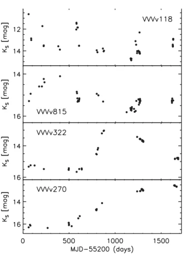
Figure 17. Examples ofKslight curves for the different classifications as
explained in the text. (top) Phased light curves of STV star with a measured period, VVVv683 and EB VVVv350. (bottom) Light curves of STV star, without a measured period, VVVv169, the fader VVVv243 and the dipper VVVv504.
the light curve of the object, thus not resembling the light curves of objects in the STV category. An exception is VVVv118, which shows four brief rises on time-scales of weeks.
The light curves in this category typically have a monotonic rise of 1 mag or more, though sometimes a lower level scatter is present atop the rising trend. In a small number of cases, the rise in the light curve is poorly sampled, starting at or before the beginning
of the time series, but the subsequent drop exceeds 1 mag. Fig.18
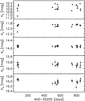
Figure 18. Examples ofKslight curves for different objects in the eruptive
classification as explained in the text. From top to bottom, we show objects VVVv118, VVVv815, VVVv322 and VVVv270.
temporal behaviour observed in objects belonging to this class. As we have already mentioned, VVVv118 shows multiple short, high-amplitude rises. In general, objects show outbursts which last between 1 and 4 yr (see VVVv815 and VVVv322). We also detect a few cases where the outburst duration cannot be measured as it extends beyond 2014 data (e.g. VVVv270).
When comparing to the behaviour of known classes of eruptive variables, VVVv118 would resemble that of EXors and VVVv270 could potentially be an FUor object (based only on photometric data). However, most of the objects have outburst durations that are in between the expected duration for EXors and FUors.
Considering the outburst duration of the known subclasses of young eruptive variables, we are likely to miss detection of FUor outbursts if they went into outburst prior to 2010. In the case of EXors, which have outbursts that last from few weeks to several months, we would expect to detect more of these objects given the time baseline of VVV. However, our results show a lack of classical EXors, which could be a real feature or it could be related to the sparse VVV sampling. Thus, we need to test our sensitivity to short, EXor-like eruptions.
We simulate outbursts with time-scales from 2 months to 3 yr. First, we generate a very rough approximation of an eruptive light
curve with outburst duration,To. The light curve consists of: (1)
A quiescent phase of constant magnitude that lasts until the begin-ning of the outburst, which is set randomly at a point within the 2010–2012 period (between 0 and 1000 d). (2) A rise which is set
arbitrarily to have a rate of 0.15 mag d−1, lastingT
rise=10 d until
reaching an outburst amplitude of 1.5 mag, which is a little below the median for the VVV eruptive variable candidates. (3) Plateau phase with a constant magnitude set to the peak of the outburst.
This phase lasts forTo−Trise−Tdecline=To−20 d. (4) The
de-cline, which lasts 10 d and has a rate of 0.15 mag d−1. Finally, (5) a
second quiescence phase. To every point in the light curve, we add
a randomly generated scatter of±0.2 mag. Once the light curve is
generated, we measure the magnitude of the synthetic object at the observation dates of a particular VVV tile. If the synthetic object
showsKs≥1 mag, then it is marked as a detection. This
proce-dure is repeated 1000 times for each outburst duration (which is set to be between 30 and 900 d). We also repeat this procedure for four different VVV tiles.
The simulation shows that the number of detections is very similar
(∼80 per cent) forTo > 7 months and declines slowly as To is
reduced, falling by a factor of 2 forTo=2 months. However, this
is not enough to cause the apparent lack of eruptive variables with EXor-like outbursts in our sample. We conclude that the longer (1–4 yr) durations that we observe are the typical values for IR eruptive variables, rather than a sampling effect.
The characteristics of our eruptive sample (seePaper II) agree
with recent discoveries of eruptive variables that show a mixture of characteristics between the known subclasses of eruptive variables
(see e.g. Aspin, Greene & Reipurth2009). We note that
classifica-tion of our sample into the known subclasses becomes even more problematic when taking spectroscopic characteristics into account, as e.g. VVVv270, the potential FUor from its light curve, shows an emission line spectrum or VVVv322 shows a classical FUor
near-IR spectrum. InPaper II, we propose a new class of eruptive
variable to describe these intermediate eruptive YSOs.
Sources classified as eruptive are very likely to be eruptive vari-ables, where the changes are explained by an increase of the ac-cretion rate on to the star due to instabilities in the disc of YSOs
(see e.g. Audard et al.2014). We find 39 objects in subgroup (a),
45 in (b) and 106 in (c). The whole class of faders/bursts represents 43 per cent of the likely YSO sample.
(iv) EBs: we find 24 objects with this light-curve morphology, representing 5 per cent of the sample. We are able to measure a possible period in 15 of them. The remaining nine objects are left with this classification given the resemblance of their light curves to the objects with measured periods. We expect that a number of them will be field EBs contaminating our YSO sample. However,
inspection of the 2–23 μm spectral index for each object,α, (see
Fig.23), indicates that 12 objects are classified as either class II
or flat-spectrum sources. If these are in fact YSOs, they would represent a significant discovery as YSO EBs are invaluable anchors for stellar evolutionary models, which generally lack empirical data
on stellar radii. Fig.19shows the light curve and location of one
candidate YSO EB, VVVv317, withP=6.85 d andα= −1.57. The
spectral index places it at the edge of the classification of class II YSOs.
In Fig. 20, we compare the amplitude distributions
(Ks,max−Ks,min) of the different categories of variable YSO. We