Modelling soil, carbon and vegetation dynamics in estuarine wetlands experiencing sea level rise

Texto completo

(1)Proceedings of 2013 IAHR Congress © 2013 Tsinghua University Press, Beijing. Modelling soil, carbon and vegetation dynamics in estuarine wetlands experiencing sea-level rise Franco Trivisonno School of Engineering, The University of Newcastle, University Drive, Callaghan, NSW 2308, Australia E-mail: [email protected] José Rodríguez School of Engineering, The University of Newcastle, University Drive, Callaghan, NSW 2308, Australia E-mail: [email protected] Gerardo Riccardi CIC-UNR, Departamento de Hidráulica and CURIHAM, Facultad de Ciencias Exactas, Ingeniería y Agrimensura, Universidad Nacional de Rosario, Riobamba 245 bis (2000) Rosario, Argentina E-mail: [email protected] Patricia Saco School of Engineering, The University of Newcastle, University Drive, Callaghan, NSW 2308, Australia E-mail: [email protected] ABSTRACT: Estuarine wetlands are among the most productive ecosystems in the world, providing unique habitats for fish and many terrestrial species. They also have a carbon sequestration capacity that surpasses terrestrial forest. In NSW, and most of south eastern Australia, they typically display a vegetation zonation with a sequence mudflats - mangrove forest - saltmarsh plains from the seaward margin and up the topographic gradient. Estuarine wetlands respond to sea-level rise by vertical accretion and horizontal landward migration, in order to maintain their position in the tidal frame. In situations in which accretion cannot compensate for sea-level rise and buffer areas for landward migration are not available, estuarine vegetation can be lost due to unsuitable hydraulic conditions. Predicting estuarine wetlands response to sea-level rise requires simultaneous modelling of water flow, soil and vegetation dynamics. This paper presents some preliminary results of our recently developed numerical model for wetland dynamics in wetlands of the Hunter estuary of NSW. The model continuously simulates tidal inputs into the wetland and vegetation types are determined based on their preference to prevailing hydrodynamic conditions. Accretion values based on vegetation types are computed and the topography is updated accordingly. The model is driven by local information collected over several years, which include estuary water levels, accretion rates, soil carbon content, flow resistance and vegetation preference to hydraulic conditions. Model results predict further wetland loss under an accelerated sea-level rise scenario and also under current conditions of moderate increase of estuary water levels. KEY WORDS: Vegetation dynamics, Estuarine wetlands, Sea-level rise. 1 INTRODUCTION In the Hunter estuary of NSW, as in most of south eastern Australia, estuarine wetlands typically comprise intertidal mudflats at the seaward margin, followed further inland first by mangrove forest and then by saltmarsh plains. Mangrove forest and saltmarsh are important for estuarine fish [Mazumder et al., 2005] and provide unique habitats for terrestrial fauna. In particular, saltmarsh is used by insectivorous bats as feeding habitat and by shorebirds as roosting habitat, clearly preferring it to mangrove forest [Saintilan and Rogers, 2006]. Estuarine wetlands are sinks for fine grained riverine sediment and can sequester carbon at higher rates than forests [Howe et al., 2009; Mitsch et al., 2012]. During periods of sea-level rise wetlands tend to maintain their relative submergence through a number of mechanisms, one of which consists of surface build-up (accretion) via sedimentation. The captured sediment has a high organic component given by roots, fallen branches and leaves, so sedimentation is effectively sequestering carbon. Since this carbon is buried, the sequestration is essentially permanent. This has prompted international initiatives to develop wetland “blue carbon” offset standards and projects certifiable by the Clean Development Mechanism or the Voluntary Carbon Standard in a similar fashion to the most traditional forest or renewable energy offsets [Danone Fund for Nature, 2010]. Predictions for most of the Australian coast of accelerated sea-level rise are particularly dangerous for estuarine wetlands comprising mangroves and saltmarsh. While in some situations mangroves can adapt quickly to changes in sea level and enhance establishment of saltmarsh by reducing wave energy and promoting sedimentation, experimental evidence gathered across Australia reveals a consistent trend of landward mangrove encroachment into saltmarsh, to a large extent related to sea-level rise [Saintilan and Williams, 1999]. Given time, it might be expected that saltmarsh would transgress landward too, occupying low-lying elevations accessed by tides only under elevated sea-level conditions. However, barriers to landward transgression -either natural or artificial- often prevent this, and the encroachment of.

(2) saltmarsh by mangrove yields a net decline in wetland area. This encroachment also results in lower habitat diversity and reduced overall wetland productivity, including reduced utilisation by shorebirds. As a result of mangrove encroachment due to a number of factors including sea-level rise and barriers, coastal saltmarsh in parts of southeast Australia has been declared an endangered ecological community. Planning for the effects of sea-level rise is therefore a major issue for governments in general and wetland managers in particular. Current coastal planning tools are mainly based on models at two different scales: national or regional and local. The national or regional scale tools are GIS based inundation models, like the Sea Level Affecting Marshes Model (SLAMM) [Park et al., 1989], with forcing functions that account for a very basic wetland dynamics. These models can be adequate for a global assessment, but the limited capacity of incorporating complex processes and the coarse resolution make them unsuitable for site-specific research or management. Local scale models are much more reliable and incorporate some of the processes, but they are typically developed for particular systems and are not easily adapted to different settings [Rogers et al., 2012]. In this paper we present preliminary results of a physically-based model that incorporates a variety of physical and biological processes and can thus be potentially used in different wetland systems. The model has been implemented in Area E of the Kooragang Wetlands (which can be seen in Figure 1), an important bird roosting site that has lost considerable areas of saltmarsh in part due to increased estuary water levels and mangrove encroachment [Howe et al., 2009, 2010; Rodriguez and Howe., in press]. 2 STUDY AREA The site for this research (Fig. 1) is a rehabilitated wetland in the Hunter Estuary, Australia, known as Area E of Kooragang Island. The site is adjacent to the Hunter Wetlands National Park and it constitutes an important shorebird roost site [Kingsford et al. 1998]. It consists of a 124 ha tidal sub-catchment with two defined inlets to the south arm of the Hunter River; one of which is an 0.45 m culvert (on Wader Creek) and the other an 8.5 m wide tidal channel (on Fish Fry Creek). The area is bounded to the east by the Kooragang Island Mainline, to the north by a water supply pipeline, and to the south and west by a levee on the north bank of the Hunter River south arm. Internal flow is hydraulically complex, with a number of culverts and roads that divide the site into four major compartments, Fish Fry Creek, Wader Creek, Wader Pond and Swan Pond (Fig. 1.b). Estuarine habitats include mangrove forest, saltmarsh, mudflat, tidal pools and tidal creeks. Fringing upland habitats include pasture and freshwater/brackish wetlands.. Figure 1 (a) The Hunter estuary and the study area, Area E; (b) detail of Area E of Kooragang Island.. Rehabilitation activity in 1995 involved the replacement of two 0.5 m diameter culverts with a bridge on Fish Fry Creek to increase tidal flushing and improve habitat for fisheries and shorebirds. These culverts were originally installed ca. 1950 to drain the wetlands for agricultural activity, principally cattle grazing. The effect of culvert removal resulted in a dramatic change to tidal conditions (i.e. tidal range and inundation regime) of the area immediately upstream of the bridge, but other areas of the wetland were less affected because of the presence of internal controls (culverts). Tidal channels in the Fish Fry Creek compartment were enlarged through erosion and mangrove colonized and displaced previous marsh areas. As a result, shorebird species were gradually excluded from the Fish Fry Creek compartment over the period 1997-2007. Increased tidal flows also promoted the landward migration of saltmarsh communities, but this was limited by existing infrastructure that acted as a barriers. By 2007, there was already a 17% net loss of saltmarsh, tidal pools and other habitats used by shorebirds [Howe et al., 2010]. An extensive set of field and remote sensing data was available for the implementation of the numerical model [Howe, 2008]. These include measurements of the general landform of the study area, the distribution of vegetation types and the spatial coordinates and physical characteristics of critical hydraulic controls, morphological characteristics of the 2.

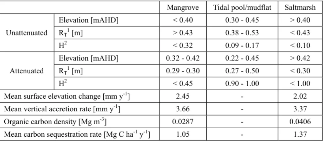
(3) dominant wetland vegetation species (A. marina, S. virginicus and S. quinqueflora), soil properties (including carbon content), soil accretion and surface elevation change, and water levels. 2 MODEL FORMULATION The proposed model includes interactions of flow-vegetation-soil processes over significant time scales. Ecogeomorphic systems like wetlands display feedbacks at different time scales -since each process evolves at its own paceand a model should be able to capture those scales [Saco and Rodríguez, 2013]. Significant changes in wetlands structure occur over decadal to centennial time scales, and previous modelling efforts have attained long simulation times at the expense of important simplifications in problem geometry or physics. As a result, their predictive capability is limited to idealized situations and cannot accommodate detailed features like culverts, bridges and manmade obstructions that can have important repercussions on wetland flow. The proposed model overcomes those limitations by using a detailed hydrodynamic description of the flow within a semi-coupled hydrodynamic-vegetation-soil evolution modular structure. 2.1 Flow module An accurate hydrodynamic description of tidal wetting and drying dictates a time discretization of the order of seconds, so a fast and efficient numerical scheme is needed if long simulation times are sought. A flood model is an ideal candidate, since it is designed to provide an immediate result during a storm event. The selected flow module is VMMHH 1.0 [Riccardi et al., 2009], a fast, two-dimensional hydrodynamic model originally designed to simulate floodplain inundation. This tool is the result of the combination of the hydrologic-hydraulic model CTSS8 [Riccardi, 2000; Stenta et al., 2008] and the Windows platform SIMULACIONES 2.0 [Stenta et al., 2005] for pre and post-processing and visualization of data and results. VMMHH 1.0 is based on the scheme of cells originally proposed by Cunge [1975], and simulates rainfall-runoff processes with multidirectional and multi-layer flow dynamics. The governing equations are those of continuity (Equation 1) and different simplifications of the momentum equation, which are transformed to obtain the discharge between the linked cells. The continuity equation at each cell can be written as: ASi dzi /dt + Pi (t) + ∑ (k=1,j) Qk,i. (1). where Pi (t) accounts for rainfall, interception, surface storage, infiltration and external flow exchange at cell i; ASi and zi are surface wetted area and water level at cell i, respectively; and Qk,i is the exchange flow rate between cell i and its j neighbouring cells. The scheme is implemented over a 2D computational grid with regular rectangular cells, which is ideal for raster DEM data. Cells can be valley-type or river-type, representing either overland or channel flow. The exchange flow Q can be computed using different discharge laws between cells, which have been derived from the momentum equation for each specific situation. In this way, discharge laws for open channel flow, bridges, weirs, culverts, junctions, changes of section, pumping stations, etc., can be incorporated into the model. For example, for links in which physical boundaries are present between cells, e.g. road embankments, the broad-crested weir equation is used. The same equation is used for links describing flow through weirs, bridges and culverts. Three types of boundary conditions can be specified: water level as a function of time, discharge as a function of time, and water level-discharge relation. Initial conditions include water levels at cells and discharges at links [Riccardi, 2000]. The model equations are solved using an implicit finite-difference scheme and the Gauss-Seidel method [Riccardi, 2000]. The stability of the scheme is based on the Courant-Friedrichs-Lewy condition, which is satisfied for the Courant number C = V dt /dx  1. V = v ± (gh)0.5 is a characteristic velocity that includes the computed flow velocity v and the celerity of surface waves (gh)0.5. Based on this condition, a 5 seconds time-step was required for the simulations presented in this paper. 2.2 Vegetation and soil evolution models Results from the hydrodynamic model are integrated over a one-year period and this information is passed on to the vegetation module. Vegetation in estuarine wetlands responds to hydrodynamic forcing via the hydroperiod (proportion of submergence time) and prevailing tidal range conditions over longer time scales, so a time step of one year is appropriate for modelling [Saco and Rodríguez, 2013]. In order to simulate saltmarsh and mangrove establishment, vegetation-specific preference values of hydroperiod and tidal range from field measurements are used. Preference values of hydroperiod and tidal range have been experimentally determined for the Hunter wetlands during spring tides [Howe et al., 2010; Rodriguez and Howe, in press] and are shown in Table 1. Vegetation class determined by the hydrodynamic variables is passed on to the soil evolution module, which computes soil accretion and surface elevation change based on experimentally-determined vegetation specific values. Soil accretion contributes to wetland soil surface elevation changes but is modulated by subsurface processes (swelling, compaction). Changes in surface elevation and in vertical accretion are determined based on previous works [Howe et al., 2009] and are also presented in Table 2. Values of topography according to vegetation cover are updated and a new hydrodynamic simulation is carried on.. 3.

(4) Table 1 Preference values of hydroperiod, tidal range and surface elevation for each vegetation type and wetland conditions, and surface elevation changes and vertical accretion rates observed for each vegetation type and wetland conditions Mangrove. Tidal pool/mudflat. Saltmarsh. Elevation [mAHD]. < 0.40. 0.30 - 0.45. > 0.40. RT1 [m]. > 0.43. 0.38 - 0.53. < 0.43. < 0.32. 0.09 - 0.17. < 0.10. Elevation [mAHD]. 0.32 - 0.42. 0.22 - 0.45. > 0.42. RT1 [m]. 0.29 - 0.30. 0.27 - 0.50. < 0.30. < 0.45. 0.90 - 1.00. < 1.00. Mean surface elevation change [mm y ]. 2.45. -. 2.02. Mean vertical accretion rate [mm y-1]. 3.66. -. 3.37. 0.0287. -. 0.0406. 1.05. -. 1.37. Unattenuated. 2. H Attenuated. 2. H. -1. -3. Organic carbon density [Mg m ] -1. -1. Mean carbon sequestration rate [Mg C ha y ] 1. 2. Spring tidal range; hydroperiod during spring tides.. Table 2 Relations used in the vegetation and soil model Mangrove. Tidal pool/mudflat. Elevation [mAHD]. -. ≥ 0.35 m + SLR. RT [m]. -. > 0.40. 1. H. ≤ 0.45 -1. 3. < 0.35 m + SLR ≤ 0.40. > 0.45. Saltmarsh 3. ≥ 0.35 m + SLR2 ≤ 0.40 > 0.45. Mean surface elevation change [mm y ]. 2.45. -. 2.02. Mean carbon sequestration rate [Mg C ha-1 y-1]. 1.05. -. 1.37. 1. Spring tidal range; 2hydroperiod during spring tides; 3expected sea-level rise according to the simulation time.. 3 MODEL SETUP The model was applied to the part of Area E where active vegetation dynamics was occurring. The VMMHH 1.0 computational mesh was constructed with the aid of available topographic data resulting in 6369 rectangular elements, each one sized 12.5 m x 12.5 m (Fig. 2). The modelled area covers 99.52 Ha and the mesh density is 0.0064 elements/m2. Three major culverts were introduced in the model (EC1, EC2 and EC3 in Fig. 2). The Fish Fry Creek’s inlet and channels to the east of the culverts were modelled using river-type cells, with all other elements considered as valley type. Hourly tidal water level was applied as a boundary condition at the Fry Fish Creek’s inlet using a one-year dataset from Ironbark Creek’s gauge, which is located 2 Km upstream of the study site on the south arm of the Hunter River. Wader Creek’s inlet was not included in the simulation as the amount of flow that conveys to the wetland is only 1 % of the total inflow [Rodriguez and Howe, in press]. Other water level boundary conditions (non-time varying) were set at the east end of culverts channels (BC1, BC2 and BC3 in Fig. 2) in order to link the modelled area to the non-modelled part of area E (most of Swan Pond). No rainfall was considered during this period. Flow resistance was represented by a Manning’s roughness coefficient n = 0.10 for all valley-type elements, while n = 0.04 was used for river-type elements. This n values can be considered averages over different vegetation substrates. Initial water levels at each element were set based on historic values. Water level data used for boundary and initial conditions as well as culverts, creek and channels dimensions were provided by previous studies [Howe, 2008; Rodriguez and Howe, in press]. Time-step for computing was set at 5 seconds, while time-step for output data printing was set at 1 hour. CPU time for the simulated period was approximately 10 hours on a Quad.i7-3770 3.40 GHz processor, representing a computing-simulation time ratio greater than 700. As explained in 2.2, abiotic variables such as hydroperiod during spring tides and spring tidal range were calculated in order to relate them to vegetation distribution. A moon phases calendar [Moon Phase Data (Geoscience Australia), 2012] was used for classifying spring-tides as 177-hour periods around new and full moon dates [Boon, 2004]. Two different scenarios for sea level rise over a 20 year-period were considered. According to observed increases in the wetland over the past 10 years [Howe et al., 2009], a medium scenario with an increment of 8 mm y-1 was set. This is also suggested by the upper end of IPCC’s 4th Assessment Report (AR4) A1FI projections, which are in line with recent global emissions and observations of sea level rise for the Hunter and Central Coast of NSW. In order to get more extreme values, a high-end scenario with an increment of 11 mm y-1 was also simulated. This case considers the possible high end risk identified in the AR4 and more specifically in post IPCC AR4 research, including the impacts of recent warming trends on ice sheet dynamics beyond those already included in the IPCC projections [OzCoasts, 2012]. As values of accretion rate and surface elevation changes (Table 1) were determined during actual changes in sea-level of 8 mm y-1 (the same sea level-rise considered by the medium scenario) values of accretion rate and surface elevation changes for the high-end 4.

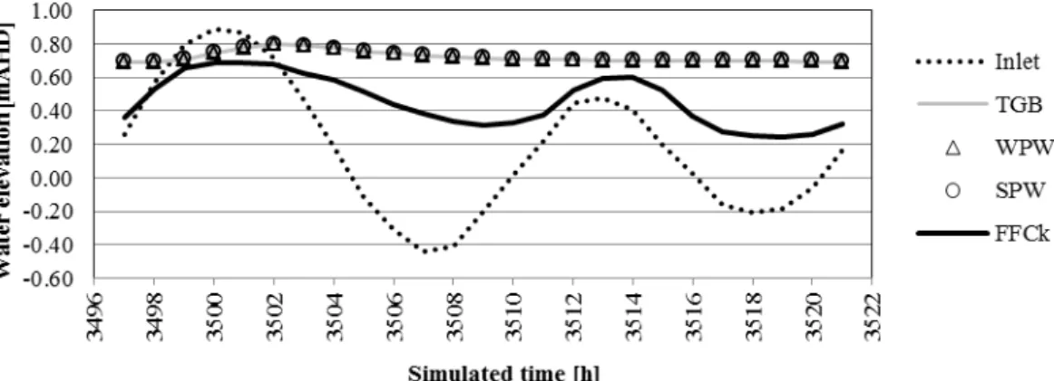
(5) scenario were adjusted proportionally.. Figure 2 Area E of Kooragang Island (© Google Earth) and model mesh, including river-type elements (in black). Also included in the figure are the locations of interest points: Fish Fry Creek’s inlet (Bridge), culverts EC1, EC2 and EC3 and reference locations for each compartment (TGB, WPW, SPW and FFCk).. 4 RESULTS AND DISCUSSION 4.1 Flow patterns Reference locations representing each one of the compartments of the wetlands were selected in the model (TGB in Wader Creek, WPW in Wader Pond, SPW in Swan Pond and FFCk in Fish Fry Creek, see Fig. 2). From observation of Figure 3 it can be seen that model results showed a remarkable tidal attenuation on certain compartments, such as Wader Creek, Wader Pond and Swan Pond. Tidal attenuation in compartments was the result of infrastructure and terrain elevation, and agrees with previous measurements and model results [Howe et al., 2010; Rodriguez and Howe, in press].. Figure 3 Water elevation evolution at reference locations during a spring tide. 5.

(6) 4.2 Vegetation distribution and surface elevation change Vegetation type in each cell was modelled, as explained in section 2.2, by comparing hydroperiod, tidal range and relative surface elevation values provided by the hydrodynamic model with the thresholds given by the vegetation module of the model (Table 2). Figure 4a shows the current observed vegetation distribution. Figure 4b shows results of vegetation distribution simulated using the model. These results were obtained from simulations of 1-year duration using the boundary water level tidal conditions at the Fly Fish Creek’s inlet described in section 3. As observed from figures 4a and 4b, the simulated vegetation distribution is in reasonably good agreement with the observed distribution. Simulations of vegetation distribution after 20 years for the two different sea level rise scenarios are presented in Figure 5. Table 2 shows the rates in mean surface elevation change for the various vegetation types used by the vegetation module in each cell. Yearly values at each cell were accumulated to simulate future surface elevation conditions over a 20-year period, and new hydrodynamic simulation was run over the updated topography. The resulting vegetation distributions based on the new values of hydroperiod, tidal range and surface elevation for the medium sea level rise-rate (8 mm y-1) and the high end level rise sea-rate (11 mm y-1) are shown respectively in Figures 5a and 5b. (a). Saltmarsh. (b). (c). Tidal pool/mudflat. Mangrove. Figure 4 (a) Actual vegetation distribution; (b) Simulated vegetation distribution for current tidal and sea level conditions.. (a). Saltmarsh. (c). (b). Tidal pool/mudflat. Mangrove -1. Figure 5 Simulated vegetation distribution corresponding to a sea-level rise rate of 8 mm y (a) and 11 mm y-1 (b) over 20-years. 6.

(7) From the analysis of Figures 4 and 5 an assessment of the capabilities and limitations of the model can be made. Firstly, the empirical thresholds on the hydraulic variables seem to be able to capture present conditions as shown by Figure 4. This is despite not including the entire wetland in the simulation domain and also not including some minor culverts and channels. The main shortcoming of this simplified description is a less accurate prediction of mangrove dynamics in the vicinity of channelized areas. The absence of channels results in increased attenuation of tidal conditions, which prevents mangrove establishment and results in an underprediction of mangrove areal extent. Regarding predictions of wetland vegetation distribution under sea level rise conditions after 20 years, both scenarios give qualitatively similar results (Figures 5a and 5b). For both scenarios tidal pool/mudflat areas expand from the centre of the wetland to its peripheral areas replacing previous saltmarsh areas, and in turn saltmarsh areas migrate to higher grounds. These effects are slightly more pronounced for the high-end sea level rise-rate. Mangrove areas are also adversely affected by sea level rise. However, it should be noticed that the absence of a few channels, currently present within the mangrove zones, may have important implications for local hydrodynamic conditions and therefore affect mangrove distribution. In particular, mangrove encroachment on saltmarsh cannot be simulated in the absence of erosional channels that promote favourable conditions. The model predicts a reduction of 6.33 % for mangrove in the medium sea level rise-rate scenario, and a reduction of 13.77 % in the high-end sea level rise-rate scenario, along with a significant reduction of saltmarsh (47.04 %) for in the medium sea level rise-rate scenario, and an even greater reduction (54.45 %) in the high-end sea level rise-rate scenario. 4.4 Carbon sequestration Carbon sequestration rates were calculated using organic carbon density values (Table 1) and computed values of accretion rates for each cell depending on vegetation type. These values were then integrated over the area occupied by each vegetation type and are presented in Table 3 for the present reference state and for the two sea-level rise scenarios. It can be seen from the table that there is a significant reduction in the carbon sequestration rate for the two sea level rise scenarios, being 36.60 % for the medium sea-level rise (8 mm y-1) and 44.01 % for the high-end scenario (11 mm y-1 sea-level rise rate). Table 3: Computed vegetation areas and carbon sequestration rates for reference year and the two sea-level rise scenarios Reference year. Medium scenario. High-end scenario -13.77 % 19.48. Mangrove area [Ha]. 22.59. 21.16. -6.33 %. Saltmarsh area [Ha]. 50.19. 26.58. -47.04 %. 22.86. -54.45 %. 26.73. 51.78. +93.71 %. 57.17. +113.88 %. 92.48. 58.63. -36.60 %. 51.78. -44.01 %. Tidal pool/mudflat area [Ha] -1. Carbon sequestration rate [Mg C y ]. 5 CONCLUSIONS A numerical model developed for analysing wetland dynamics in wetlands of the Hunter estuary of NSW, which involves a hydrodynamic module and a soil-vegetation module that are sequentially linked, has been shown able to predict vegetation distribution in the wetlands. Using two different sea-level rise rate scenarios of 8 mm y-1 and 11 mm y-1 vegetated area losses ranged from 6.33 % to 13.77 % for mangrove and from 47.04 % to 54.45 % for saltmarsh, respectively. This resulted in a significant reduction of the carbon sequestration rate of the wetland. The reduction is 36.60 % for the lower sea level rise scenario and 44.01 % for the higher sea level rise scenario. Evolution of vegetation distribution outputs given by model runs confirms the expected response of estuarine wetlands to sea-level rise: saltmarsh areas migrate inland in order to maintain a favourable position in the tidal frame, but in parts of the wetlands buffer areas for landward migration are not available and saltmarsh-vegetated area is replaced by tidal pool/mudflat. Improvements in results could be obtained with a more detailed definition of model domain: an extension of modelled area in order to include the entire wetland is needed, along with the inclusion of non-modelled creeks, inlet and infrastructure such as levees and some minor culverts. Finally, impacts of setting different roughness coefficient to each cell according to the assigned vegetation type were not studied in this paper and they could result in improved predictive capabilities of this modelling approach. ACKNOWLEDGEMENT The first author acknowledges the financial support of the University of Newcastle through a Postgraduate Scholarship.. 7.

(8) References Boon, J. D. (2004) Secrets of the Tide: Tide and Tidal Current Analysis and Predictions, Storm Surges and Sea Level Trends, v. 2005: West Sussex, Horwood Publishing Limited, 212 p. Cunge, J. (1975) Two dimensional modelling of flood plains, in: Mahmood K. and Yevjevich V., eds., Unsteady flow in open channels, Water Resources Publications, Fort Collins, 705-762. Danone Fund for Nature (2010) Achieving Carbon Offsets through Mangroves and Other Wetlands. November 2009 Expert Workshop Meeting Report, ed. Nick Davidson. Danone Group/IUCN/ Ramsar Convention Secretariat, Gland, Switzerland. 87pp. Howe, A., Rodríguez, J. F. and Saco, P. M. (2009) Vertical accretion and carbon sequestration in disturbed and undisturbed estuarine wetland soils of the Hunter estuary, southeastern Australia. Estuarine Coastal and Shelf Science 84, 75–83. Howe, A., Rodríguez, J.F., Spencer, J., MacFarlane, G. and Saintilan, N. (2010) Response of estuarine wetlands to reinstatement of tidal flow. Marine and Freshwater Research, 61: 702-713. Kingsford, R. T., Ferster Levy, R., Geering, D., Davis, S. T., and Davis, J. S. E., 1998, Rehabilitating Estuarine Habitat on Kooragang Island for Waterbirds, including Migratory Wading Birds (May 1994 - May 1997), NSW National Parks and Wildlife Service, 105 p. Mazumder, D., Saintilan, N., and Williams, R. J. (2005) Temporal variations in dish catch using pop nets in mangrove and saltmarsh flats at Towra Point, NSW, Australia. Wetlands Ecology and Management, 13: 457-467. Mitsch, W.J., Bernal, B., Nahlik, A., Mander, Ü., Zhang, L., Anderson Christopher, J., Jørgensen, S. and Brix, H. (2012) Wetlands, carbon and climate change. Landscape Ecology, 1-15. Moon Phase Data (2012) Australian Government, Geoscience Australia, Earth Monitoring and Reference Systems, Astronomical Information. Website: http://www.ga.gov.au/earth-monitoring/astronomical-information/moon-phase-data.html OzCoasts: Australian Online Coastal Information (2012) Geoscience Australia, Australian Government. Website: http://www.ozcoasts.gov.au Park, R.A., Trehan, M.S., Mausel, P.W. and Howe, R.C. (1989) The effects of sea level rise on U.S. coastal wetlands. In The Potential Effects of Global Climate Change on the United States, J.B. Smith and D.A. Tirpak (Eds.). Report to Congress, U.S. Environmental Protection Agency, Washington, DC. Riccardi, G.A. (2000) A model of cells for hydrological-hydraulic modeling. Journal of Environmental Hydrology, Vol.8, Paper 15, November 2000. Riccardi, G., Zimmermann, E., Basile, P., Stenta, H., Scuderi, C. and Rentería, J. (2009) Rehidrología y modelo de pronósticos arroyos Ludueña y Saladillo. Informes de avance 1, 2, 3 y 4. Rosario, Argentina: Convenio FCEIAMASP, 2009, 583 pp. Riccardi, G., Stenta, H., Scuderi, C., Basile, P., Zimmermann, E. and Trivisonno, F. (2013) Aplicación de un modelo hidrológico-hidráulico para el pronóstico de niveles de agua en tiempo real. Tecnologia y Ciencias del Agua, Vol. IV, Núm. 1, enero-marzo de 2013. Rodriguez, J.F. and Howe, A. (in press) Estuarine wetland ecohydraulics and migratory shorebird habitat restoration. Book chapter to appear in Ecohydraulics, an Integrated Approach, Maddock, I., Harby, A., Kemp, P., Wood, P. (Eds.). John Wiley and Sons, UK. Rogers, K., Saintilan, N. and Copeland, C. (2012) Modelling wetland surface elevation dynamics and its application to forecasting the effects of sea-level rise on estuarine wetlands. Ecological Modelling, 244: 148-157. Saco P.M., and Rodríguez J.F. (2013) Modeling Ecogeomorphic Systems. In Treatise on Geomorphology, Vol 2, Quantitative Modeling of Geomorphology, Shroder John F. (Editor-in-chief), Baas, A.C.W. (Volume Editor), Academic Press San Diego, pp. 201-220. Saintilan, N., and Williams, R. J. (1999) Mangrove transgression into saltmarsh environments in south-east Australia. Global Ecology and Biogeography, 8: 117-124. Saintilan, N., and Rogers, K. (2006) Coastal wetland elevation trends in southeast Australia. Catchments to Coast. Society of Wetland Scientists 27th International Conference, 42-54. Stenta, H., Rentería, J. and Riccardi, G. (2005) Plataforma computacional para gestión de información en la simulación hidrológica-hidráulica del escurrimiento superficial. XX Congreso Nacional del Agua y III Simposio de Recursos Hídricos del Cono Sur, Mendoza, Argentina, vol. 1, CD, núm. T74, 2005, 13 pp. Stenta, H., Riccardi, G. and Basile, P (2008) Influencia del grado de discretización espacial en la respuesta hidrológica de una cuenca de llanura mediante modelación matemática distribuida. Ingeniería Hidráulica en México. Vol. XXIII, núm. 3, julio-septiembre de 2008, pp. 123-138.. 8.

(9)