DEA as a business failure prediction tool

Application to the case of galician SMEs

Abstract

In the research group we are working to provide further em-pirical evidence on the business failure forecast. Complex fit -ting modelling; the study of variables such as the audit impact on business failure; the treatment of traditional variables and ratios have led us to determine a starting point based on a ref-erence mathematical model. In this regard, we have restricted the field of study to non-financial galician SMEs in order to develop a model1 _{to diagnose and forecast business failure. We}

have developed models based on relevant financial variables from the perspective of the financial logic, voltage and finan -cial failure, applying three methods of analysis: discriminant, logit and multivariate linear. Finally, we have closed the first cycle using mathematical programming –DEA or Data Envel-opment Analysis– to support the failure forecast. The simulta-neous use of models was intended to compare their respective conclusions and to look for inter-relations. We can say that the resulting models are satisfactory on the basis of their capacity for prediction. Nevertheless, DEA contains significant points of criticism regarding its applicability to business failure. Keywords: DEA operational research, business failure, fore-cast

Pablo de Llano Monelos University of A Coruña pdellano@udc.es

Carlos Piñeiro Sánchez University of A Coruña carpi@udc.es

Manuel Rodríguez López University of A Coruña carpi@udc.es

DEA como herramienta en el pronóstico del fallo empresarial. Aplicación al caso de las Pyme gallegas

Resumen

Este grupo de investigación busca aportar mayor evidencia del pronóstico del fracaso em-presarial. La construcción de modelos de ajuste complejos, el estudio de variables tales como el impacto de la auditoría en el pronóstico del fracaso, así como el tratamiento de variables y ratios clásicas nos lleva a determinar un punto de partida mediante la construc-ción de un modelo matemático que sirva de referencia. En este sentido, hemos reducido el ámbito de estudio a Pyme no financieras gallegas con el fin de desarrollar un modelo que permita diagnosticar y pronosticar el fracaso empresarial. Hemos desarrollado los modelos con base en variables financieras relevantes desde la óptica de la lógica financiera, la ten -sión y el fracaso financiero, aplicando tres metodologías de análisis: discriminante, logit y lineal multivariante. Por último, hemos cerrado el primer ciclo, utilizando la programación matemática DEA (Data Envelopment Analysis) con el fin de fundamentar la determinación del fracaso. El uso simultáneo de los modelos se explica por la voluntad de comparar sus respectivas conclusiones y buscar elementos de complementariedad. La capacidad de pronóstico lograda nos permite afirmar que los modelos obtenidos son satisfactorios. No obstante, el DEA presenta determinados puntos críticos significativos en cuanto a su apli -cabilidad al pronóstico del fallo empresarial.

Palabra clave: investigación operativa DEA, fracaso empresarial, pronóstico.

Introduction

Business failure in its different manifestations –bankruptcy, temporary

insolven-cies, bankruptcy proceedings, mergers and spin-offs– is a recurrent topic in fi -nancial literature for its theoretical importance and for its serious consequences

for economic activity. We are currently seeing an inexplicable fluctuation and

creditors, employees, etc. Direct costs associated with business failure in the ju-dicial environment represent an average 5% of the company’s book value. Also,

indirect costs connected with loss of sales and profits, the growth of credit cost (risk premium), the impossibility to issue new shares and the loss of investment opportunities increase that cost to nearly 30%.2 _{Therefore, it is important to detect}

the possibility of insolvency in its first stages.

The first contributions date back to Beaver (1966), Altman (1968) and Ohlson

(1980), who examined different methodological alternatives to the development of explanatory and forecast models for these events. The most traditional approach has been enriched with the development of alternative models, more reliable and less dependent on methodological, determining factors; among them, we can hi-ghlight the logit and the probit analyses; the recursive portioning techniques and

several characteristic forms of artificial intelligence –both expert systems and ne

-tworks of artificial brain cells, as well as support vector machines. The complex and unstructured nature of the analysis also justifies the application of heuristic

methods such as computer-assisted techniques of social decision and, of course, fuzzy logic models.

Business failure

The research of business failure in its different manifestations –bankruptcy, tem-porary insolvencies, bankruptcy proceedings, mergers and spin-offs– is a recurrent

topic in financial literature for its theoretical importance and for its serious con -sequences for the economic activity. Several alternative methodologies have been

discussed on the basis of the first contributions of Beaver (1966), Altman (1968) and Ohlson (1980) in order to develop explanatory and predictive models for these

events. The most traditional approach, materialised in the initial studies by Altman

(Altman, 1968; Altman et al., 1977; Altman, 2000; Altman et al., 2010), has been enriched with the development of alternative models, perhaps more reliable and less dependent on methodological, determining factors; among them, we can

high-light the logit and the probit analyses (Martin, 1977; Ohlson, 1980; Zmijewski,

1984); the recursive portioning techniques (Frydman et al., 1985) and several

char-acteristic forms of artificial intelligence –both expert systems and networks of arti

-ficial brain cells (Messier and Hansen, 1988; Bell et al., 1990; Hansen and Messier,

1991; Serrano and Martín del Brio, 1993; Koh and Tan, 1999; Brockett et al., 2006),

as well as support vector machines (Shin et al., 2005; Härdle et al., 2005). The

complex and unstructured nature of the analysis also justifies the application of

heuristic methods such as computer-assisted techniques of social decision (level-3 GDSS, for example Sun and Li, 2009) and, of course, fuzzy logic models (Dubois

and Prade, 1992; Slowinski and Zopounidis, 1995; McKee and Lensberg, 2002).

The first formal study of the business failure based on explanatory models was performed by Beaver (1966), who analysed the phenomenon with the help of the financial logic and the information provided by the financial statements. Beaver’s approach (1966) provides an expanded vision of the business failure concept per

-fectly consistent with the modern financial approach, although suffering from the

inherent limitations of his statistical methodology.

Altman (1968) is the reference antecedent in the application of the multivariate

approach to the business failure issue: he suggested the development of

discrimi-nant models that, apart from the proper classification, could become de facto stan -dards and contribute to enhancing the objectivity of the solvency analysis. Howe-ver, the implementation of MDA is conditioned by its scenario, particularly, by the requirement that factors should be distributed in accordance with a normal model

–something that, as is known, is at least arguable in the case of financial ratios– and

by the fact that the (failed and solvent) subpopulations should be homoscedastic.

Due to its mathematical approach, the discriminant models do not provide specific

information to determine the causes and internal structure of the failed event, even when they [are] re-estimated for several time windows (De Llano et al., 2010, 2011abc).

Ohlson (1980) used the logit approach, which was originally used by Martin (1977), to assess the solvency of financial entities, and generalised it for a more ge

-neral case: the non-financial companies. He improves Martin’s original approach

(1977) thanks to a theory that estimates the probability of failure in an industrial

company on the basis of four basic attributes: dimension, financial structure, finan -cial performance and liquidity. Beyond the methods, the logit approach is in line with the idea that business failure is not a dichotomous event, as Altman’s MDA approach showed, but a complex gradable phenomenon. That is precisely why a

comprehensive classification may be less relevant and significant than the measu

chosen for this dependent variable. Altogether, logit models have proved to be at

least as efficient as MDA. Finally Ohlson (1980) confirmed that combining purely accounting information with external and market indicators allows for a signifi -cant improvement of the explanatory and predictive capacity of models, as well

as providing the first indications that financially distressed companies tend to get

involved in formal irregularities (such as delays in annual account deposits or the

accumulation of qualifications) and minimise the flow of information even beyond

the legally required standards (Piñeiro et al., 2011).

The development and validation of these models have provided valuable evidence,

not only to better understand the causes and evolution of the financial and structural

processes that lead to failure but also to identify key variables and indicators that

directors and external users should control in order to infer the existence of finan -cial dysfunctions and forecast possible default or insolvency events. Here we must

highlight a small number of financial ratios related to liquidity, profitability and the

circulation of current assets and liabilities (Rodríguez et al., 2010), and also macro-economic factors (Rose et al., 1982), proxies related to management quality (Peel et al., 1986; Keasey and Watson, 1987), and qualitative indicators related to the audit

of accounts (Piñeiro et al., 2011).

It is precisely because of the failure events that the design and contrast of

em-pirical models tend to emphasise their capacity to identify financially distressed

companies. Therefore, the validation seems to have been aimed at enhancing the capacity to prevent type II errors (to wrongly assume that a faltering and

potentia-lly failed company is financiapotentia-lly healthy). A still unsolved question refers to the

precise study of false positives, i.e. the study of solvent companies classified as potentially failed. Ohlson (1980) draws attention to the abnormally low error rates

observed in earlier studies (especially in Altman’s MDA models), as later research has shown divergences that are not explained in the type I and type II (de Llano et al., 2010). Due to reasons that may be rooted in the sampling or the method itself, models seem to achieve outstanding results among failed companies unlike the solvent companies, suggesting that they tend to overestimate the probability of

failure: the rate of healthy companies qualified as potentially failed is significantly high, at least when compared to the type I error rate. Our experience shows that these biased opinions are concentrated in companies that share specific financial characteristics because of, for example, the nature of their activity, financial and

This issue is closely connected to the initial calibration of the model as well as

the later analysis of its coefficients (Moyer, 1977; Altman, 2000). But besides its statistical relevance, a type I error has an enormous practical significance for the company, as it undermines lenders’ and market confidence, and it may also under

-mine the company’s financial standing, driving it to an eventual insolvency, which

otherwise would not have happened.

In recent years a number of models based on the Data Envelopment Analysis (DEA) have been developed to forecast business failures and compare these

re-sults with those achieved through other techniques such as the Z-Score (Altman) or the LOGIT (Olshon). The logistic regression technique uses the cut-off point of 0.5 for the classification (potential failure probability, cut-off point to rate the

cases). In terms of probability, this means that the companies who are over the cut-off point are solvent and the ones who are not are insolvent. As Premachandra3

pointed out, the LOGIT cut-off point of 0.5 is not appropriate for the classification of both failed and non-failed companies when using the DEA efficiency analysis. He said that efficiency scores in DEA analyses can be too slant, especially when using super-efficient DEA models. Therefore, if we use the DEA analysis as a tool

to forecast business failure, we should use an adjusted discriminant analysis or an evaluating function, establishing values between 0.1 and 0.9 for the cut-off point. There are many studies in the literature where the logistic regression –or probit– is

used to forecast business failures. They are methods based on separating the fit

sample from the contrast sample.

Data Envelopment Analysis (DEA)

Data Envelopment Analysis (DEA),4 5 _{called frontier analysis, is one of the} li-near programming applications. This is a mathematical programming technique to measure the performance of groups of economic or social structures within the

same industry sector. DEA purpose is to measure the efficiency of each organi -sational unit by translating the available data into multiple results explaining its

efficiency: the degree of input-efficiency. Due to the high number of relevant va

-riables, it is difficult for the manager to determine which components of the orga

-nisation are actually efficient. Efficiency will be determined by the ratio between

the monetary value of the output (ur) and the monetary value of the input (v_i):

Defined in this manner, efficiency expresses the conversion ratio of inputs to outputs. The closer the coefficient is to 1, the higher the degree of efficiency will be for the organisation assessed. One limitation of this efficiency measurement system is that prices must be identical, otherwise the com

-parison cannot be considered to be fair. The efficiency values for each analysed

element must be between 0 and 1. The construction of the mathematical

program-ming model requires to define the objective function, which will be the result of

maximising the total value of the final products:6 _{The model}

only generates one restriction, where outputs are equal to the inputs for all the companies analysed . It appears that we are being taken away

from the financial target of having an efficient company if the value of its Outputs

(u_r) is higher than the value of its Inputs (v_i). What we are trying to determine is the

value that makes the company (E=1) efficient. Consequently, the company that is not efficient will have a lower value (E<1). Notwithstanding the trivial interpreta -tion of “how can it be possible that the output is lower than the input?” it is clear that _{does not work for us as it means that} , which in PL terms is the same as saying that . The solution algorithm aims to wear out the limits of restrictions, therefore, to cancel h. In this case, the associated shadow price will (most likely) be positive. We also know that this means that if it was possible to in-crease the corresponding input available by one unit we would be able to inin-crease the output volume by one unit too. Thus:

• It makes sense to demand because it is coherent with the logic of the PL model regarding minimising the surpluses, which in this case means

an inactive production capacity associated to good financial standings.

This idea implied in the investment models: performed projects equal to

resources available and, the good financial standing reflecting inactive

funding –which we will try to minimise.

• The ideal maximum would be achieved when all the good financial

standings were cancelled, which would mean to maximise the use of the

resources. This production unit, i.e. this company, would be the efficiency

paradigm and would be standing in that imaginary frontier resulting from the model.

• In terms of duality, this ideal maximum allows us to evaluate the mixture and the degree of use of the resources, assigning them a price. It is interesting to observe that, the way they are now, these optimal conditions are a similar concept to the theoretical relation of balance between the revenues and the marginal costs –the marginal cost is that one caused by the increase of the limit of restriction while the marginal income is the increase of the output, precisely, the shadow price. Again, the maximum refers to I’ = C’, i.e. to output = input.

In 1993 Barr, Seiford and Siems released a tool to measure the managerial efficien

-cy of banks based on financial and accounting information. The model used banks’ essential functions of financial intermediation to determine a tool to measure their

productivity. The traditional way to measure productivity is the ratio of the multi-ple outputs and inputs.

We use the term DMUs for Decision Making Units. Perhaps we should try to turn it into a worldlier term and talk about the elements we wish to compare: Depart-ments; Companies; Transportation; Communications; etcetera, or any other ele-ment/unit we wish to compare to another or others of its peers. Thus, if we consider that we have m inputs and s outputs, the DMU will explain the given transfor-mation of the input m in the output s as a measure of productivity (efficiency).

The literature about investments has been focused on the study of models with measurable variables. That’s why in the last decades we found a few new models covering the need for including all those variables that take part in the decision making process regarding investments but that are not being considered because of their intangible nature.

Troutt (1996) introduced a technical note based upon three assumptions: mono -tonicity of all variables, convexity of the acceptable set and no Type II errors (no

false negatives). They use an efficient frontier that is commonly used in various fi

-nancial fields. Essentially, DEA can be used just to accept or reject systems as long

as all the variables are conditionally monotone and the acceptable set is convex.

Retzlaff-Roberts (1996) stresses two seemingly unrelated techniques: DEA and

rela-tive efficiencies, whenever the relevant variables are measurable. On the contrary,

the discriminant analysis is a forecast model such as in the business failure case.

Both methods (DEA – DA) aim at making classifications (in our case, of failed and

healthy companies) by specifying the set of factors or weights that determines a particular group membership relative to a “threshold” (frontier).

Sinuany-Stern (1998) provides an efficiency and inefficiency model based on the

optimisation of the common weights through DEA, on the same scale. This me-thod, Discriminant DEA of Ratios, allows us to rank all the units on a particular

unified scale. She will later review the DEA methodology along with Adler (2002),

introducing a set of subgroups of models provided by several researchers, and

ai-med at testing the ranking capacity of the DEA model in the determination of effi

-ciency and ineffi-ciency on the basis of the DMUs. In the same way, Cook (2009)

summarises 30 years of DEA history. In particular, they focus on the models

me-asuring efficiency, the approaches to incorporate multiplier restrictions, certain

considerations with respect to the state of variables and data variation modelling.

Moreover, Chen (2003) models an alternative to eliminate non-zero slacks while

preserving the original efficient frontier.

There have been many contributions in recent years, of which we can highlight Sueyoshi (2009), who used the DEA-DA model to compare Japanese machinery

and electric industries, R&D expenditure and its impact in the financial structure

of both industries. Premachandra (2009) compares DEA, as a business failure pre-diction tool, to logistic regression. Liu (2009), with regards to the existing search

for the “good” efficient frontier, tries to determine the most unfavourable scenario, i.e. the worst efficient frontier with respect to failed companies, where ranking the worst performers in terms of efficiency is the worst case of the scenario analy -sed. Sueyoshi and Goto (2009a) compare the DEA and DEA-DA methods from

the perspective of the financial failure forecast. Sueyoshi and Goto (2009b) use DEA-DA to determine the classification error of failed companies in the Japanese construction industry. Sueyoshi (2011) analyses the capacity of the classification

by combining DEA and DEA-DA, as in (2011a) on the Japanese electric industry. Finally, Chen (2012) extends the application of DEA to two-stage network

structu-res, as Shetty (2012) proposes a modified DEA model to forecast business failure

Thirty years of DEA

It has been thirty years since Charnes, Cooper and Rhodes released their model to

measure efficiency in 1978, a model that is used to compare efficiency between

several units, departments, companies and tools. It is a technique that allows us to

determine relative efficiency and that requires to have quantitative capacity: inputs

at their price, outputs at their price.

In 2009, Cook and Seinford released an article containing the evolution of DEA from 1978 to 2008, as just a DEA evolution overview and its state of the art. Re-garding business failure, the really important thing is the union of DEA with the DA phenomenology; DEA adversus DEA-DA. Before discussing the modelling

and results, we should note that DEA is just used to determine relative efficiency.

Therefore, it is not an instrument that can be used to classify “in or out of,” yes/no,

“before or after;” as DEA measures relative efficiency, not maximum or optimal efficiency despite its being based on linear programming optimisation.

Proposal

In order to contrast the model, we have taken a sample of small and medium size galician enterprises, which have been put into two categories: failed and healthy. Despite not showing in detail the very different causes why the companies got into

financial troubles, the sample has the strength of being objective and guaranteeing a comprehensive classification for all the companies, which is essential for the

application of the several analysis methods (MDA, Logit, and DEA). The use of

more flexible criteria is undoubtedly an option to consider to refine the system since it shows more accurately specific situations of insolvency such as the return

of stocks. Nevertheless, the special features of these situations bring forward an element of subjectivity, as there are several sources of information (RAI, BADEX-CUG, etc.), not all of them compatible.

We have had access to the official accounting information of 75 640 galician com

-panies between 2000 and 2010. Out of them, three hundred and eighty-four (384) are in a situation of bankruptcy or final liquidation, thereby, there are 298 left with

Likewise, we have managed to get 107 healthy companies – galician SMEs that in the last years have “always” had an audit report rated as “pass,” and that have

been used to determine the models LOGIT, MDA and the efficiency contrast DEA.

Selection of the explanatory variables

The particular problem raised by the election of the forecast variables is a

signi-ficant issue because of the lack of a well-established business failure theory. The

consequential use of experimental subgroups means that results cannot be compa-red either transversely or temporarily. The choice of the explanatory variables has

been based on two principles: popularity in the accounting and financial literature, and frequency and significance level in the most relevant studies on business fai -lure forecast. In all cases, ratios have been calculated on the basis of the indicators recorded in the Annual Accounts without introducing adjustments previously ob-served in the literature, such as marking-to-market or the use of alternative accoun-ting methods.

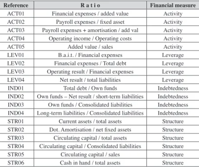
Table 1 Financial ratios

Reference R a t i o Financial measure

ACT01 Financial expenses / added value Activity ACT02 Payroll expenses / fixed asset Activity ACT03 Payroll expenses + amortisation / add val Activity ACT04 Operating income / Operating costs Activity

ACT05 Added value / sales Activity

LEV01 B.a.i.t. / Financial expenses Leverage LEV02 Financial expenses / Total debt Leverage LEV03 Operating result / Financial expenses Leverage LEV04 Net result / total liabilities Leverage IND01 Total debt / Own funds Indebtedness IND02 Own funds – Net result / short-term liabilities Indebtedness IND03 Own funds / Consolidated liabilities Indebtedness IND04 Long-term liabilities / Consolidated liabilities Indebtedness STR01 Current assets / total assets Structure STR02 Dot. Amortisation / net fixed assets Structure STR03 Circulating capital / total assets Structure STR04 Circulating capital / Consolidated liabilities Structure STR05 Circulating capital / sales Structure

Reference R a t i o Financial measure

STR07 Net result / Circulating capital Structure STR08 Asset decomposition measure Structure LIQ01 Operating cash flow / total assets Liquidity LIQ02 Operating cash flow / Consolidated liabilities Liquidity LIQ03 Operating cash flow / short-term liabilities Liquidity LIQ04 Operating cash flow / sales Liquidity LIQ05 Operating cash flow / total assets Liquidity

LIQ06 Operating cash flow / total liabilities Liquidity LIQ07 Operating cash flow / short-term liabilities Liquidity LIQ08 Cash flow, resources generated / sales Liquidity LIQ09 Cash in hand / current liabilities Liquidity LIQ10 Stock / short-term liabilities Liquidity LIQ11 Stock + realizable / short-term liabilities Liquidity

LIQ12 No credit interval Liquidity

LIQ13 Realizable / short-term liabilities Liquidity

PRO01 B.a.i.t. / total assets Profitability PRO02 B.a.i.t. / sales Profitability PRO03 Net result / sales Profitability PRO04 Net Result-realisable– Stock / total assets Profitability PRO05 Net result / total assets Profitability PRO06 Net result / Own funds Profitability ROT01 Current assets – Stock / sales Rotation

ROT02 Stock / sales Rotation

ROT03 Sales / Receivables Rotation

ROT04 Sales / Current assets Rotation

ROT05 Sales / fixed asset Rotation

ROT06 Sales / total assets Rotation

ROT07 Sales / Circulating capital Rotation

ROT08 Sales / Cash in hand Rotation

SOL01 Current assets–Stock / short-term liabilities Solvency

SOL02 Current assets / Total debt Solvency

SOL03 Current assets / current liabilities Solvency

SOL04 Fixed asset / Own funds Solvency

SOL05 Consolidated liabilities / total assets Solvency

SOL06 Own funds / total assets Solvency

SOL07 Own funds / fixed assets Solvency

SOL08 Short-term liabilities / total assets Solvency

SOL09 Profit before tax / short-term liabilities Solvency TES01 Cash flow / current liabilities Treasury

Significant variables: LEV₀₄, ROT₀₆, SOL₀₆, LIQ₁₂, PRO₀₅, LIQ₀₅, IND₀₃, STR₀₃.

On the basis of the preceding considerations, the related MDA, MRL models7 _were determined with the following results:8

Table 2

MDA prediction (BD2a may 2010)

Table 3

LOGIT prediction (BD2a may 2010)

7_{De Llano et al. (2010, 2011a, b, c).}

8_{YB, yb: Year Before the failure: 1YB one year before the failure, 2YB two years before, 3 YB three years before,}

4YB four years before, GLOBAL four years altogether.

Forecasts for

failed s/(H, F) 1yb 2yb 3yb 4yb 5yb 6yb 7yb 8yb 9yb 10yb 11yb

MDA 1 YB

Forecast 96.3% 94.6% 93.9% 92.3% 91.0% 91.7% 90.7% 89.4% 85.9% 82.0% 80.2% MDA 2 YB

Forecast 93.7% 94.0% 92.0% 90.4% 89.8% 91.3% 91.6% 89.7% 85.8% 87.0% 87.9% MDA 3 YB

Forecast 98.1% 98.8% 98.4% 98.1%97.6% 100.0% 96.3% 98.0% 96.2% 97.5% 96.7% MDA 4 YB

Forecast 90.7% 90.6% 85.4% 85.8% 84.0% 83.3% 86.7% 84.7% 81.0% 85.4% 85.7%

MDA GLOBAL

Forecast 90.3% 84.8% 84.0% 82.8% 82.4% 81.7% 77.2% 79.8% 77.6% 78.0% 82.4%

Forecasts for failed

s/(H. F) 1yb 2yb 3yb 4yb 5yb 6yb 7yb 8yb 9yb 10yb 11yb

LOGIT 1 YB

Forecast 81.8% 87.3% 87.9% 87.5% 85.0% 82.4% 84.5% 86.6% 83.6% 78.1% 70.0%

LOGIT 2 YB

Forecast 65.8% 58.2% 54.5% 54.3% 45.6% 48.3% 39.3% 42.1% 41.5% 30.2% 31.9%

LOGIT 3 YB

Forecast 78.6% 70.8% 64.0% 62.3% 57.2% 59.6% 48.9% 52.0% 48.7% 44.7% 50.0%

LOGIT 4 YB

Forecast 76.8% 81.8% 77.1% 76.6% 75.3% 72.5% 69.8% 70.9% 68.9% 62.0% 65.9%

LOGIT GLOBAL

Table 4

MRL prediction (BD2a may 2010)

The capacity for forecasting business failure featured by any of the above models is satisfactory, with the result obtained by the MDA adjustment being the most ac-ceptable. The linear model appears to have a good prediction capacity but we must rule it out because of its inability to classify healthy companies in an acceptable manner.

The contrast against the 2011 database, BD2b, resulted in:

Table 5

MDA/LOGIT prediction (BD2b nov 2011)

Forecasts for

failed s/(H, F) 1yb 2yb 3yb 4yb 5yb 6yb 7yb 8yb 9yb 10yb 11yb

MRL 1 YB

Forecast 85.0% 95.8% 96.6% 98.8% 98.4% 96.7% 99.5% 99.5% 100.0% 98.8% 98.9% MRL 2 YB

Forecast 75.5% 89.3% 93.5% 93.5% 94.1% 91.3% 94.4% 94.4% 95.6% 94.4% 96.7% MRL 3 YB

Forecast 81.8% 93.4% 96.5% 97.7% 97.2% 97.0% 98.6% 98.5% 97.8% 97.5% 98.9% MRL 4 YB

Forecast 71.8%86.4% 88.0% 88.0% 87.9% 87.1% 90.5% 89.9% 90.4% 89.9% 85.7%

MRL GLOBAL

Forecast 92.6%95.9% 97.3% 98.4% 97.7% 97.5% 98.1% 98.5% 98.4% 96.8%100.0%

Failed in % 1yb 2yb 3yb 4yb 5yb 6yb 7yb 8yb 9yb 10yb 11yb

MDA 1YB 98% 97% 94% 90% 92% 91% 92% 89% 89% 84% 84%

MDA 2YB 94% 95% 91% 87% 91% 90% 89% 90% 88% 87% 87%

MDA 3YB 99% 99% 98% 96% 97% 99% 97% 98% 97% 97% 98%

MDA 4YB 95% 95% 90% 91% 91% 91% 91% 90% 89% 89% 89%

MDA

GLOBAL 97% 97% 95% 93% 94% 96% 95% 93% 96% 92% 98% LOGIT 1YB 87% 88% 86% 85% 86% 85% 83% 85% 82% 80% 78%

LOGIT 2YB 70% 63% 57% 54% 51% 51% 45% 43% 46% 37% 38%

LOGIT 3YB 84% 74% 66% 63% 64% 63% 55% 57% 53% 49% 54%

LOGIT 4YB 88% 86% 75% 72% 74% 70% 68% 71% 66% 64% 61% LOGIT

GLOBAL 65% 48% 51% 51% 53% 51% 52% 51% 47% 48% 50%

Data (average

in No.) 113 119 297 295 273 256 236 215 195 173 122

Failed

(average) 88% 84% 80% 78% 79% 79% 77% 77% 75% 73% 74%

Solvent

Previously to the estimation of models, we have performed a factor analysis aimed at reducing the variables to a small number of synthetic and homogenous regres-sors. We perform the estimation for each of the time horizons, between one and four years before the failure event. In all cases we have excluded the factors whose eigenvalue was lower than one.

In the four horizons, the four variables with more weight are related to profitability

and liquidity (which is measured as cash flow), indebtedness and solvency; the composition of the factors is similar with the exception of the year 4 before the

fai-lure (4yb). These results confirm the relationship between the ratios of profitability and operating cash flow (Gombola and Ketz, 1983; Pina, 1992).

Table 6

LOGIT, MDA, MRL Contrast s/107 healthy companies (2010 BD3a)

The prediction capacity of the MDA and LOGIT adjustments on the healthy com

-panies should be understood from two different perspectives. On one hand, they

lack quality when it comes to rank healthy companies as non-failed in comparison

to their better performance when contrasting failed companies. On the other, the contrast of the financial statements reveals that healthy companies have, or may have in the future, certain imperfections. One of the first conclusions referred to the

dismissal of MRL (Linear Regression) models on the basis of their poor prediction capacity.

Forecasts for

healthy s/(H, F) 1yb 2yb 3yb 4yb 5yb 6yb 7yb 8yb 9yb 10yb 11yb

MDA 1 YB 39.3% 37.4% 43.9% 43.9% 44.9% 47.7% 45.8% 43.9% 46.7% 53.3% 48.1% MDA 2 YB 43.9% 36.4% 40.2% 36.4% 41.1% 39.3% 42.1% 38.3% 38.3% 42.9% 43.3%

MDA 3 YB 9.3% 11.2% 8.4% 5.6% 8.4% 9.3% 8.4% 10.3% 7.5% 8.6% 10.6%

MDA 4 YB 42.1% 33.6% 35.5% 24.3% 29.9% 31.8% 35.5% 33.6% 33.6% 28.6% 34.6% MDA GLOBAL 32.7% 26.2% 28.0% 23.4% 28.0% 27.1% 25.2% 24.3% 24.3% 21.9% 21.2%

LOGIT 1 YB 16.8% 20.6% 18.7% 18.7% 21.5% 27.1% 22.4% 23.4% 27.1% 28.6% 28.8%

LOGIT 2 YB 73.8% 81.3% 87.9% 91.6% 92.5% 88.8% 89.7% 90.7% 89.7% 90.5% 91.3%

LOGIT 3 YB 83.2% 81.3% 83.2% 86.9% 89.7% 89.7% 86.0% 86.0% 82.2% 85.7% 86.5%

LOGIT 4 YB 68.2% 71.0% 80.4% 80.4% 82.2% 83.2% 79.4% 76.6% 72.9% 77.1% 82.7%

LOGIT GLOBAL 75.7% 77.6% 77.6% 77.6% 82.2% 81.3% 77.6% 80.4% 76.6% 74.3% 76.9%

MRL 1 YB 3.7% 2.8% 0.0% 0.0% 0.0% 0.0% 0.0% 0.0% 0.0% 0.0% 0.0%

MRL 2 YB 14.0% 12.1% 1.9% 3.7% 2.8% 1.9% 1.9% 0.9% 1.9% 1.9% 2.9%

MRL 3 YB 0.0% 0.0% 0.0% 0.0% 0.0% 0.0% 0.0% 0.0% 0.0% 0.0% 0.0%

MRL 4 YB 20.6% 20.6% 2.8% 5.6% 3.7% 3.7% 3.7% 3.7% 5.6% 3.8% 3.8%

Contrast with DEA model

With the aim of unifying criteria, we have taken the ratios shown below on the

basis of the financial-accounting information available from the 298 failed and 107 healthy companies:9

Outputs

It shows the level of indebtedness with respect to the total assets. The higher this value is, the more externally dependent the company will be and, consequently, will restrict its room for manoeuvre. It explains the risk of insolvency (business failure).

It shows the need for immediate cover; possibility of default on its short-term liabilities. The higher its value is, the lower the liquidity will be and the higher the risk of insolvency.

Inputs

Ratio explaining the asset capacity to generate income (ROA).

It reveals how efficient the company is concerning the use of

its own resources to generate liquidity (cash).

It reveals how efficient the company is concerning the use of its own resources to generate profit before interest and tax, i.e. it is the capacity to generate profit by the asset irrespectively of how it has been funded.

It reveals the capacity to profit before interest and tax

in order to cover debt and operating costs on EBIT.

It reveals the added value ratio earned by the sharehold-ers, although we should use the market value, but SMEs are not usually quoted on the stock exchange; hence this substitution in the denominator.

Warehouse, Debtors, Treasury and other short-term liabili-ties, i.e. Current Assets. The higher the ratio is the higher the liquidity will be and, therefore, the greater the capacity to meet short-term obligations will be too.

It shows that long-term resources are funding short-term liabilities. The circulating capital is the difference between current assets and liabilities. The higher it is, the better. However, an “excessive” value would be a

sign of idle resources. In addition, we could find “false negatives” as under certain financial structures the average maturity of the suppliers’ credits is higher than the

average maturity of the debtors’ credits, i.e. a negative circulating capital. But let’s take the ratio in a strictly protective sense to cover short-term liabilities, therefore, it should always be positive (CC=FM=Ac-Pc>0).

Without entering into the debate about the choice of the above ratios, we have

made the MDA and LOGIT adjustments on our original samples, in the last five

Table 7

LOGIT, MDA Prediction

While they are still good adjustments, the quality of the adjustment is

questiona-ble, to say the least, given the little significance of some of the ratios used in the

mentioned articles.

DEA model

DEA aims to determine the hyperplanes defining a closed surface or Pareto fron

-tier. Those units (companies, DMUs) located on the border will be efficient, as all the others will be inefficient. The DEA model10 _{will include the variable c}

k, to allow variable returns models.

LOGIT MDA

Fail Variables Type Classified _correctly Fail Variables Type Classified _correctly

Year 0

All H 75.70%

Year 0

All H 46.70%

F 94.60% F 92.20%

Excluded (O2, I6) H 76.60% Excluded (I1, I2, _{I5, I6, I7)} H 42.10%

F 94.90% F 91.90%

Year -1

All H 67.30%

Year -1

All H 78.50%

F 94.60% F 81.00%

Excluded (O2,

I3, I4)

H 66.40% Excluded (I1, I3, I4, I5)

H 77.60%

F 93.90% F 80.30%

Year -2

All H 64.50%

Year -2

All H 85.00%

F 92.40% F 57.00%

Excluded (I4) H 64.50% Excluded (I2, _{I3, I4)} H 84.10%

F 92.40% F 81.10%

Year -3

All H 50.50%

Year -3

All H 80.40%

F 90.50% F 79.40%

Excluded (I1, I2, I3, I4, I5)

H 51.40% Excluded (I1, I2,

I3, I4, I5)

H 83.20%

F 91.20% F 79.40%

Year -4

All H 69.20%

Year -4

All H 65.40%

F 93.90% F 89.30%

Excluded (O2,

I3, I4)

H 70.10% Excluded (O2, I1,

I3, I4, I5, I6)

H 65.40%

F 94.70% F 90.40%

Equation 1: DEA for efficient frontier

Based on the linear programming system, we have determined the set of

hyper-planes defining the efficient and inefficient frontiers. We must put forward one criticism, as the determination of the efficient frontier offers scope for arbitrari -ness. It is based on the average value of the ratios, the best adjustment, and the best regression. In our case, we took the average values of the ratios for each year (Healthy and Failed). Therefore, this is a “relative” frontier, not absolute. Thus,

we have determined both efficient and inefficient frontiers for each of the last four years. On the basis of the above approach, we have determined both the efficient and inefficient units depending on the particular case. In the case of two variables,

the frontiers could be displayed as follows below:

Figure 1

Since we have been able to determine the set of DMUs defining the efficiency fron

-tiers, the likelihood of financial failure or non-failure, we can add a complementary approach in order to determine whether any DMU analysed is or not efficient.

Equation 2: additive DEA

The above determined frontiers11 _{provide the parameters for a hyperplane or} ma-trix of inputs (X) and outputs (Y), which will be formed by the values of the

varia-bles (ratios) that make up the set of efficient companies and that is located on this hypothetically efficient line (hyperplane)12

• X will be a matrix of kxn inputs and Y, a matrix of mxn outputs, with n being the number of DMUs making up the frontier, including their respective k inputs, m outputs,

• e is an unit vector,

• x₀ , y₀ : column vectors showing the inputs and outputs of the DMU subject

to classification,

• s- _s+ _{: vectors showing the slacks of the matrix of inputs and outputs in the}

DMU analysed, indicating the relative efficiency; the lower the objective

function is the better the position of DMU will be with respect to the

frontier (efficient/inefficient),

• l _{will be the vector determining the intensity of development in the analysed}

unit with respect to the efficient (or inefficient, where appropriate) frontier. Since we have been able to determine the efficient/inefficient hyperplane, the next

step will be to determine whether an analysed unit is or not on the frontier. This will allow us to determine the stress levels in a particular unit with respect to the

11_{Equation 1.}

hypothetically efficient/inefficient ones. This is a more complex and tedious task

as we will have to develop each and every analysed unit in order to place it in

re-lation to the efficient or inefficient frontier.

This is the second step, the development of the approach shown in equation 2.

Based on a given efficient/inefficient frontier formed by the matrixes Xl_{, Y}l_{, we}

will analyse a particular company (DMU0) represented by its inputs and outputs (x₀,y₀)’. The result will tell us the state of the company with respect to the efficient and inefficient frontiers, respectively.

In our case, based on the three databases discussed above, four efficient frontiers (EF) and other four inefficient (nonEF) ones were created in relation to the four years analysed. The database containing 2 966 (Healthy and Failed) companies

was randomly sampled, with 402 (failed and non-failed) companies evaluated with

respect to the efficient and inefficient frontiers, achieving the following results:

Table 8

DEA-based classification

We can state that capacity to classify the analysed companies (DMUs) is

signi-ficantly high. The column “Classified correctly” shows that they are not on the Pareto, or efficient, frontier but not too far from it, therefore, we do not know how inefficient they are. We cannot forget to mention that the maximum we established

as a measure of comparison is itself “relative,” not an “absolute” measure,

althou-gh we can define it as a “relative maximum.” The “no feasible solution” indicator shows the amount of input-output vectors to be compared with respect to the effi -cient frontier, which does not have a feasible solution, i.e. it provides a solution but fails with model restrictions.

Classified

correctly Erroneously classified No feasible solution

On efficient

frontier HealthyFailed 80.54%76.39% 6.01%6.29% 13.45%17.32%

On inefficient

Figure 2

Classification in relation to efficient/inefficient frontiers

Conclusions

With this study we have sought to provide evidence showing that the statistical

models currently used to infer situations of financial distress and to forecast a pos

-sible financial failure might have overestimated the failure probability. Our earlier studies showed evidence supporting the ability of the MDA and LOGIT models to efficiently detect failed and insolvent companies. These models have now been

applied to a contrasting random sampling exclusively made up of healthy compa-nies in order to verify the possible existence of systematic biased opinions in the forecast. Likewise, the present study provides reasonable evidence about the reli-ability of the DEA model to forecast business failure. Not exempt from criticism or, if preferred, easy –immediate– applicability to the day-to-day practice of risk estimation.

In sight of the results shown above, we can confirm that DEA provides further ev -idence about whether a company is failing, thus, performing at a satisfactory level

despite its arduous modelling. On a general basis, results show that a significant ratio of the companies that we assume are failed can correctly be “classified” as

failed by the MDA, LOGIT and DEA models. But although DEA “works,” it still has significant inconveniences along with evident benefits.

Among the “benefits,” we can highlight:

• DEA can be modelled for multiple inputs and outputs

• In DEA the Decision-Making Units (DMUs) can be compared against a peer or combination of peers

• In DEA, inputs and outputs can have a different measurement, for example,

investment on R&D against efficiency and effectiveness of the production

system in terms of redundant processes found and removed

• Regarding the “inconveniences,” we should bear in mind that:

• DEA cannot eliminate the extremely technical noise, even the symmetrical

noise with zero mean that causes significant estimation errors

• DEA is good at estimating the relative efficiency of a Decision-Making Unit (DMU) but it converges very slowly to absolute efficiency. In other

words, it can tell you how well you are doing compared to your peers but not compared to a theoretical maximum.

• Since DEA is a nonparametric technique, statistical hypotheses are difficult

and also the main focus of a lot of research

• There is a significant computing problem as a standard formulation of DEA

creates a separate linear program for each DMU

We must remember that, essentially, DEA is based on a comparison exercise

be-tween peers that has been extrapolated to a “hierarchical” issue applied to financial

environments with business failure risk: “healthy” / “failed.”

Perhaps the most complex issue regarding its applicability roots is the fact that the set of articles we have been discussing are not truly academic or exclusively

academic. In a few cases they are even detached from a significant practical reality. Occasionally, its mathematical and cryptic levels make it difficult to implement in everyday life of financial management, who are aiming to determine the risk

exposure.

In addition to the great advantages of the ratios (we can visualise immediately the correct or incorrect position of our company structure; compare our company to the relevant industry, the position of other companies at the same time as our com-pany’s life cycle) there are also limitations that need to be borne in mind:

• The existing correlation between the variables forming a ratio. Something that is not implicit in the ratio concept but that subsists as an element that distorts its values and their development (i.e. its usefulness) is the potential correlation between the variables related by a ratio. This problem is aggravated with clo-sely related ratios, invalidating its reading temporarily either for being depen-dant or for a high degree of correlation. In the present case:

• Clearly-related TDTA and CLTA inputs; Total Debt, Current Debt, both types of debt with respect to the Total Assets (net assets)

• NITA, CFTA, EBTA, EBFE outputs containing elements related; Net income, Cash Flow, EBIT. Sometimes dependent, as in EBTA, where the numerator BAIT and the denominator Financial Expenses are part of the EBIT.

• The reference Values or standards: we have to take into account that ratios are control tools (objective against result), while any reference value should be established depending on the company, the sector of activity and the moment in the company’s life cycle. The evolution of the ratio and the corrective measures against deviations should take priority in the analysis.

Furthermore, we have corroborated the existence of systematic biased opinions

supporting the situations of insolvency: models perform more efficiently when

their aim is to identify potentially failed companies and they commit more er-rors on average when they are used to evaluate solvent companies. This tendency seems to be more pronounced in the discriminant models, perhaps because they impose a discretional treatment to a particular reality –the state of insolvency– that

is diffuse and liable to qualifications. In our opinion, logit models are more reliable

to grasp the different realities that coexist in the generic concept of solvency. That

is why they also perform relatively well between financially healthy companies.

It seems reasonable to conclude that DEA (based on LOGIT), MDA and LOGIT

models should not be interpreted as mutually exclusive alternatives, but as

com-plementary methods that, implemented in conjunction, can help fill their respective

gaps.

improve with the help of complementary information that may corroborate –and what it seems more important to us, qualify– the forecast. In this sense, the infor-mation provided by the audit report13 _{seems to have a special informational content} through indirect indicators such as the auditor turnover rate, the average duration

of their contracts and the proportion of qualified reports.

We must look back at the concept of “management responsibility” in the failure process. A recent study14 _{states that “two out of three Spanish senior executives} do not match up to the requirements of their responsibilities,” and also notes that “only 22% of middle managers think that senior executives are qualified to make

sensible decisions.” When the economic situation is buoyant, it is reasonable to believe that errors, the lack of leadership, the delay in the taking of decisions are easily covered by the surplus generated by the system. But what happens when the

system shrinks? The good times have hidden the low profiles of the directors. The

recession or contraction periods reveal inability to make decisions. This is not a

new idea but the verification of the “Peter Principle,” i.e. the verification of how

important the human capital is in this process. The concept of a company as a sys-tem allows us to adopt an analytical approach to identify problems, i.e. the way all the company decisions are related to each other. Formally considered, a company

is defined in Business Economics as an organisation: a complex, target-driven,

socio-technical system that also has an authority structure, a system to allocate responsibilities and a control mechanism. In the last few years we have seen many examples of an irresponsible lack of control by companies and public authorities that has resulted in the recent crises. There is no need to legislate more, just exer-cise more control; by comparing objective to result, determining the variances that have occurred, implementing corrective actions. Simple models are the most

efficient: principle of parsimony.

References

Adler, N., L. Friedman and Z. Sinuany-Stern (2002). Review of Ranking in the

Data Envelopment Analysis Context. European Journal of Operational Re-search (140): 249-265.

Altman, E. (1968). Financial Ratios, Discriminant Analysis and Prediction of Cor -porate Bankruptcy. Journal of Finance: 589–609.

 (2000). Predicting Financial Distress of Companies: Revisiting the

Z-Score and ZETA Models. Working Paper. NYU Salomon Center, july.

, R. C. Haldeman, P. Narayanan (1977). ZETA Analysis. A New Mo -del to Identify Bankruptcy Risk Corporations. Journal of Banking and Fi-nance, june: 29-54

, N. Fargher and E. Kalotay (2010). A Simple Empirical Model of

Equity-Implied Probabilities of Default. Working Paper. Available from: http://pages.stern.nyu.edu/~ealtman/DefaultModel2010JFI.pdf

Barr, R. S., L. M., Seiford and T. F. Siems (1993). An Envelopment-Analysis Ap-proach to Measuring the Management Quality of Banks. Annals of Opera-tions Research (38): 1-13.

Beaver, W. H. (1966). Financial ratios as predictors of failure. Empirical Research

in Accounting from. Journal of accountant Research (4): 71-111

Bell, T. B., G. S. Ribar and J. Verchio (1990). Neural Nets versus Logistic Regres-sion: A Comparison of Each Model’s Ability to Predict Commercial Bank Failures. En R. P. Srivastava (ed.). X Auditing Symposium Deloitte & Tou-che. Symposium on Auditing Problems. Kansas: 29-53.

Blay, A. (2005). Independence threats, litigation risk, and the auditor’s decision process. Contemporary Accounting Research (22): 759-789.

Brockett, P., L. Golden, J. Jang and C. Yang (2006). A comparison of neural net

-work, statistical methods, and variable choice for life insurers’ financial dis -tress prediction. The Journal of Risk and Insurance 73 (3): 397-419.

, W.W. Cooper, B. Golany and L. Seiford (1985). Foundations of Data

Envelopment Analysis form Pareto-Koopmans Efficient Empirical Produc -tion Func-tions. Journal of Econometrics (30): 91-107.

Chen, Y., H. Morita and J. Zhu (2003). Multiplier Bounds in DEA via Strong Com -plementary Slackness Condition Solution, International Journal of Produc-tion Economics (86): 11-19.

, L. Liang and J. Xie (2012). DEA model for Extended Two-stage

Network Structures. Omega (40): 611-618.

Cook, W.D. and L.M. Seiford (2009). Data Envelopment Analysis (DEA) – Thirty

Years On. European Journal of Operation Research (192): 1-17.

Dubois, D. and H. Prade (1992). Putting rough sets and fuzzy sets together. In In-telligent Decision Support. En R. Slowinski (ed.). Handbook of Applications

and Advances in Rough Set Theory, Kluwer Academic. Dordrecht: 203–232.

Frydman, H., E. I. Altman and D. L. Kao (1985). Introducing Recursive

Partition-ing for Financial Classification: The Case of Financial Distress. The Journal of Finance 40 (1): 269-291.

Hansen, J. and W. Messier (1991). Artificial neural networks: foundations and

application to a decision problem. Expert Systems with Applications (3): 135–141.

Härdle, W., R. Moro and D. Schäfer (2005). Predicting Bankruptcy with Support Vector Machines. Discussion Paper nº 009, 2005. SFB 649, Economic Risk. Available from: http://sfb649.wiwi.hu-berlin.de/papers/pdf/SFB

-649DP2005-009.pdf

Keasey, K. and R. Watson (1987). Non-Financial Symptoms and the Prediction of Small Company Failure. A Test of Argenti’s Hypotheses. Journal of Busi-ness Finance and Accounting 14 (3): 335-354.

Liu, F.F. and C.L. Chen (2009). The Worst-Practice DEA Model with Slack-Based Measurement. Computers & Industrial Engineering (57): 496-505.

Llano, P. de and C. Piñeiro (2011). Elementos fundamentales de dirección finan -ciera. Andavira Editorial.

 and M. Rodríguez (2011a). Contraste de los modelos de pronóstico del fallo empresarial en las pymes sanas gallegas. XXV Congreso de AE-DEM. Valencia.

 (2011b). Modelos de pronóstico del fallo empresarial en las Pymes sanas gallegas. XXV Congreso de AEDEM. Valencia.

 _{(2011c). A model to forecast financial failure, in non-financial Gali}

-cian SMEs. XII Iberian-Italian Congress of Financial and Actuarial Math-ematics. Lisbon.

Martin, D. (1977). Early Warning of Bank Failure: a Logit regression approach. Journal of Banking and Finance 1 (3): 249-276.

Matsumura, E., K. Subramanyam and R. Tucker (1997). Strategic auditor behaviour and going-concern decisions. Journal of Business Finance and Accounting (24): 77 - 759.

McKee, T. and T. Lensberg (2002). Genetic programming and rough sets: a hybrid

approach to bankruptcy classification. European Journal of Operational Re-search (138): 436-451.

Messier, W. and J. Hansen (1988). Inducing rules for expert system development: an example using default and bankruptcy data. Management Science 34 (12): 1403–1415.

Moyer, R. C. (1977). Forecasting Financial Failure: A Reexamination. Financial Management 6 (1): 11-17.

Ohlson, J. (1980). Financial Ratios and Probabilistic Prediction of Bankruptcy.

Otto, W. (2010). La alta dirección a examen. Available from:

http://www.ottowal-ter.com/prensa/pdf_invest/Estudio_OW_2010.pdf

Peel, M. J., D. A. Peel and P. F. Pope (1986). Predicting Corporate Failure. Some Results for the UK Corporate Sector, Omega. The International Journal of Management Science 14 (1): 5-12.

Pindado, J., R. Rodrigues and C. de la Torre (2008). Estimating Financial Distress Likelihood. Journal of Business Research (61): 995–1003.

Piñeiro, C., P. de Llano and M. Rodríguez (2011). Fracaso empresarial y auditoría de cuentas. XXV Congreso de AEDEM. Valencia. (Premio FESIDE a la me-jor ponencia de Investigación en Finanzas).

Premachandra I.M., G.S. Bhabra and T. Sueyoshi (2009). DEA as a tool for bank-ruptcy assessment: a comparative study with logistic regression technique. European Journal of Operational Research (193): 412–424.

Retzlaff-Roberts, D.L. (1996). Relating Discriminant Analysis and Data Envel

-opment Analysis to One Another. Computers Operations Research 23 (4): 311-322.

Robinson, D. (2008). Auditor Independence and Auditor-Provided Tax Service:

Evidence from Going-Concern Audit Opinions Prior to Bankruptcy Filings.

Auditing: a Journal of Practice & Theory 27 (2): 31–54.

Rodríguez, M., P. de Llano and C. Piñeiro (2010). Bankruptcy Prediction Models in Galician companies. Application of Parametric Methodologies and Artifi -cial Intelligence. International Conference on Applied Business & Econom-ics (ICABE 2010). A Coruña.

Rose, P. S., W. T. Andrews and G. A. Giroux (1982). Predicting Business Failure: A Macroeconomic Perspective. Journal of Accounting Auditing and Finance, Fall: 20-31.

Ruiz, E. and N. Gómez (2001). Análisis empírico de los factores que explican la mejora de la opinión de auditoría: compra de opinión y mejora en las prác-ticas contables de la empresa. Revista Española de Financiación y Contabi-lidad , XXXVI (134): 317-350

Schwartz, K. and K. Menon (1985). Auditor switches by failing firms. Accounting

Review (60): 248 - 261.

Schwartz, K. and B. Soo (1995). An Analysis of form 8-K disclosures of auditor

changes by firms approaching bankruptcy. Auditing: A journal of Practice & Theory 14 (1): 125 – 136.

Serrano, C. and B. Martín (1993). Predicción de la quiebra bancaria mediante el

empleo de redes neuronales artificiales. Revista Española de Financiación y Contabilidad 22 (74): 153-176.

Shetty, U., T.P.M. Pakkala and T. Mallikarjunappa (2012). A Modified Directio -nal Distance Formulation of DEA to Assess Bankruptcy: An Application to IT/ITES Companies in India. Expert Systems with Applications (39): 1988-1997.

Shin, K., T. Lee and H. Kim (2005). An application of support vector machines in bankruptcy prediction model. Expert Systems with Applications (28): 127 – 135.

Sinauny-Stern, Z. and L. Friedman (1998). DEA and the Discriminant Analysis of

Ratios for Ranking Units. European Journal of Operational Research (111): 470-478.

Slowinski R. and C. Zopounidis (1995). Application of the rough set approach to

Sueyoshi, T. and M. Goto (2009). Can R&D Expenditure Avoid Corporate Bank-ruptcy? Comparison Between Japanese Machinery and Electric Equipment Industries Usin DEA-Discriminant Analysis. European Journal of Opera-tion Research (196): 289-311.

 (2009a). Methodological Comparison between DEA (data

envelop-ment analysis) and DEA–DA (discriminant analysis) from the Perspective of Bankruptcy Assessment. European Journal of Operation Research (199):

561-575.

 _{(2009b). DEA-DA for Bankruptcy-based Performance Assessment:}

Misclassification Analysis of Japanese Construction Industry. European Journal of Operation Research (199): 576-594.

 _{(2011). A combined use of DEA (Data Envelopment Analysis) with}

Strong Complementary Slackness Condition and DEA–DA (Discriminant Analysis). Applied Mathematics Letters (24): 1051-1056.

 _{(2011a). Efficiency-based rank assessment for electric power indus}

-try: A combined use of Data Envelopment Analysis (DEA) and DEA-Dis-criminant Analysis (DA). Power System, IEEE Transactions on Energy

Economic 19 (2): 919-925.

Sun, J. and H. Li (2009). Financial distress early warning based on group decision making. Computers & Operations Research (36): 885 – 906.

Troutt, M.D., R. Arun and Z. Aimao (1996). The Potential use of DEA for Credit

Applicant Acceptance Systems. Computer Operations Research, Elsevier Science Ltd. 23 (4): 405-408.

Tucker, R. R. and E. M. Matsumura (1998). Going concern judgments: an econom-ic perspective. Behavioral Research in Accounting (10): 197-218.