Hydrodynamic modelling of tidal currents at Chacao Channel for a preliminary energy resource assessment

Texto completo

(1)PONTIFICIA UNIVERSIDAD CATOLICA DE CHILE ESCUELA DE INGENIERIA. HYDRODYNAMIC MODELLING OF TIDAL CURRENTS AT CHACAO CHANNEL FOR A PRELIMINARY ENERGY RESOURCE ASSESSMENT. NILS ERIK MIGUEL LINDEEN DE LA FUENTE. Thesis submitted to the Office of Research and Graduate Studies in partial fulfillment of the requirements for the Degree of Master of Science in Engineering. Advisor: RODRIGO CIENFUEGOS. Santiago de Chile, January, 2012 2012, Nils Erik Miguel Lindeen De la Fuente.

(2) PONTIFICIA UNIVERSIDAD CATOLICA DE CHILE ESCUELA DE INGENIERIA. HYDRODYNAMIC MODELLING OF TIDAL CURRENTS AT CHACAO CHANNEL FOR A PRELIMINARY ENERGY RESOURCE ASSESSMENT. NILS ERIK MIGUEL LINDEEN DE LA FUENTE. Members of the Committee: RODRIGO CIENFUEGOS CRISTIAN ESCAURIAZA CRISTOPHER AIKEN VLADIMIR MARIANOV. Thesis submitted to the Office of Research and Graduate Studies in partial fulfillment of the requirements for the Degree of Master of Science in Engineering Santiago de Chile, March, 2012.

(3) To. my. family,. Postgraduate accompanied process.. ii. teachers. colleagues me. through. and who this.

(4) ACKNOWLEDGEMENTS First of all I would like to thank my family for having supported my decision to enter the Master’s degree, over immediately getting in the labor life. It was definitely a good decision. Next, I want to thank Rodrigo Cienfuegos for his patience and lessons, and Cristopher Aiken for his constant willingness and support in the learning process of ROMS model, both helping me overcome all the obstacles that appeared on the way. Without them this process would have been much harder. As well, a great acknowledgement to Domenico Sciolla and Cristian Escauriaza for sharing their knowledge and discoveries in the flowturbine interaction area of the project, which was a tremendous help to understand certain large scale phenomena. I would also like to congratulate and thank the renewable energies company Hydrochile for the scholarship they gave me to develop my thesis, which is part of an R&D project they are managing and financing. Not many companies take these initiatives, which are definitely necessary for the development of sustainability and innovation. Last but not least, I would like to thank all the students, teachers and staff at the Hydraulics and Environmental Engineering Department at the “Universidad Católica”, for two very entertaining and enriching years as a Postgraduate student, which I will never forget without a doubt.. iii.

(5) CONTENTS Page DEDICATORY ............................................................................................................ ii ACKNOWLEDGEMENTS ........................................................................................ iii CONTENTS ................................................................................................................ iv TABLES INDEX ....................................................................................................... vii FIGURES INDEX ..................................................................................................... viii RESUMEN.................................................................................................................. xi ABSTRACT ............................................................................................................... xii 1.. INTRODUCTION .............................................................................................. 1 1.1 Context ....................................................................................................... 1 1.2 Objectives ................................................................................................... 2. 2.. BASIC FUNDAMENTS AND REVISION ....................................................... 4 2.1 Tides ........................................................................................................... 4 2.1.1 Basic Concepts and Astronomic Forcing ........................................ 4 2.1.2 Tidal Reference Levels .................................................................... 7 2.1.3 The Equilibrium Theory of Tides .................................................... 9 2.1.4 The Dynamic Theory of Tides ....................................................... 14 2.1.5 Tidal Level Prediction ................................................................... 15 2.1.6 Tidal Classification ........................................................................ 16 2.2 Tidal Energetic Flow Models ................................................................... 17 2.2.1 Tidal Energetic Resource ............................................................... 18 2.2.2 Tidal Farm Design ......................................................................... 23 2.3 Chacao Channel and the Southern Fjords ................................................ 30 2.3.1 Existent studies and papers ............................................................ 31 2.3.2 Available Data in the Channel ....................................................... 35 iv.

(6) 3.. ROMS HYDRODYNAMIC MODEL ............................................................. 38 3.1 Basic Flow Equations ............................................................................... 38 3.2 Pre-Process ............................................................................................... 40 3.2.1 Model Compilation ........................................................................ 41 3.2.2 Open and Closed Boundaries......................................................... 41 3.2.3 Bathymetry .................................................................................... 42 3.2.4 Grid Generation ............................................................................. 43 3.2.5 Time-step ....................................................................................... 45 3.2.6 Tides .............................................................................................. 45 3.2.7 Model Period ................................................................................. 46 3.2.8 Other Parameters ........................................................................... 47 3.3 Process...................................................................................................... 47 3.4 Post-Process ............................................................................................. 48. 4.. CHILEAN INLAND SEA AND CHACAO CHANNEL HYDRODYNAMICS50 4.1 2D ROMS Regional Model ...................................................................... 50 4.1.1 Bathymetry .................................................................................... 50 4.1.2 Limits ............................................................................................. 51 4.1.3 Sensitivity Analysis ....................................................................... 52 4.1.4 Model Grid..................................................................................... 57 4.1.5 Period ............................................................................................. 58 4.1.6 Model Calibration .......................................................................... 59 4.2 2D ROMS Chacao Channel Model .......................................................... 59 4.2.1 Limits ............................................................................................. 59 4.2.2 Bathymetry .................................................................................... 60 4.2.3 Model Grid..................................................................................... 63 4.2.4 Nesting Process .............................................................................. 63 4.2.5 Model Calibration .......................................................................... 64. 5.. RESULTS AND DISCUSION ......................................................................... 65 5.1 Regional Model ........................................................................................ 65 5.1.1 Tidal Components Comparison ..................................................... 65 5.1.2 Tidal Resonance............................................................................. 66 5.2 Chacao Channel Model ............................................................................ 68 v.

(7) 5.2.1 Hydrodynamics in the Chacao Channel......................................... 68 5.2.2 Chacao Channel Characteristics .................................................... 73 5.2.3 Profile Analysis ............................................................................. 75 5.2.4 Potential Estimation ....................................................................... 78 5.3 Recommendations for Future Instrumental Installation ........................... 80 6.. CONCLUSIONS .............................................................................................. 84 6.1 Regional Model ........................................................................................ 84 6.2 Chacao Channel Model ............................................................................ 84 6.3 Future Considerations .............................................................................. 85. REFERENCES........................................................................................................... 87 APPENDICES ........................................................................................................... 91 Appendix A: ROMS MANUAL ................................................................................ 92 Appendix B: ROMS MODEL COMPILATION ROUTINES .................................. 97 Appendix C: ROMS MODEL RUNNING OPTIONS ............................................ 123. vi.

(8) TABLES INDEX Page. Table 2-1: Summary of available tidal height measurements in modeled area. (Herrera, 2010). ............................................................................................................................... 37 Table 2-2: Summary of available velocity measurements in modeled area. (Herrera, 2010). ............................................................................................................................... 37 Table 4-1: Toy models characteristics for varying grid size. ........................................... 53 Table 4-2: Model characteristics for varying modeling length. ....................................... 55 Table 4-3: Sensitivity results for tidal components at Manao and Tique. ....................... 57 Table 5-1: Measured and modeled comparison of main tidal components. .................... 66. vii.

(9) FIGURES INDEX Page Figure 2-1: Tidal astronomical forcing interaction. ........................................................... 7 Figure 2-2: Main tidal reference levels, according to Chilean Navy rules. (SHOA, Glosario de Mareas y Corrientes (Publicación SHOA N° 3013), 1992) ........................... 8 Figure 2-3: Solar-Lunar interaction as a tidal generator. ................................................. 10 Figure 2-4: Tides at Longyearbyen 1-31 October 2006. a) Only M2, b) M2+S2, c) M2+S2+N2, d) M2+S2+N2+K1. Full Moon 7 Oct., New Moon 22 Oct. Lunar perigee 6 Oct. and apogee 19 Oct. Day starts at midnight UT (GMT). (Gjevik, 2006). ................. 13 Figure 2-5: World tidal patterns and the amphidromic points. ........................................ 15 Figure 2-6: Channel of variable cross-section, which connects two basins with different tidal elevations. (Garret & Cummins, 2005). ................................................................... 20 Figure 2-7: Power extraction as a function of the nth exponential and non-dimensional turbine drag (λ). (Garrett & Cummins, 2007). ................................................................. 21 Figure 2-8: Mean power density maps along (a) the northern and (b) the southern coasts of Georgia with labeled high tidal streampower density (>500 W/m) areas. (Defne, Haas, & Fritz, 2011) ................................................................................................................... 23 Figure 2-9: Definition sketch for a single turbine in a channel (Garrett & Cummins, 2007). ............................................................................................................................... 24 Figure 2-10: Tuning and power at optimal tuning for an inertial channel,. 0. 0 . (a). Optimal tuning, r3opt ( , N R* ) . (b) Fraction of a channel’s potential available for production, P avail / P max . (Vennell, 2010). ....................................................................... 26 Figure 2-11: Tidal farm model. (Lee, Jang, Lee, & Hur, 2010)....................................... 27 Figure 2-12: Results of tidal farm model, which show how at a downstream distance of 3D optimal turbine efficiency is obtained. (Lee, Jang, Lee, & Hur, 2010)...................... 27 Figure 2-13: Arrangements of turbines in a channel and the dimensions studied to study their efficiency. (Myers & Bahaj, 2012). ......................................................................... 28. viii.

(10) Figure 2-14: Model results of a dual single row arrangement of turbines over velocity deficit. (Myers & Bahaj, 2012). ....................................................................................... 29 Figure 2-15: Longitudinal centerline velocity deficits for the two row turbine arrangement. (Myers & Bahaj, 2012). ............................................................................. 30 Figure 2-16: Characteristics of three top energetic tidal channels in Chile, where Chacao Channel is by far the most attractive alternative. (Garrad-Hassan, 2009). ...................... 31 Figure 2-17: Detailed map of the CIS, including a description of main channels and gulfs. (Aiken, 2008). ........................................................................................................ 32 Figure 2-18: Diagram of tide level differences between both sides of Chacao Channel. 33 Figure 2-19: Amplitude (upper) and phase (lower) of a damped channel harmonically forced at its open end. The dashed curves indicate the modeled amplitude of M2 in the nCIS. For the solid curves, r/ω= 0.3. (Aiken, 2008). ....................................................... 34 Figure 2-20: Schematic representation of the along-channel mean flow at Remolinos Rock transect. Outflow (gray arrows) and inflow (black arrows) regions are separated by strong convergences or lateral shears represented by the dashed lines. (Cáceres, ValleLevinson, & Atkinson, 2003). .......................................................................................... 35 Figure 2-21: Available current and tide measurements in Chacao Channel. (Herrera, 2010). ............................................................................................................................... 36 Figure 3-1: Diagram of ROMS grid structure. ................................................................. 44 Figure 4-1: Detail of SHOA nautical charts available in the region. (SHOA, Cartas y Publicaciones Náuticas (Publicación SHOA N° 3000), 2010). ....................................... 51 Figure 4-2: Sketch of model limits, open boundaries and tidal wave entrance. .............. 52 Figure 4-3: Comparison of tidal resonance effect over varying grid sizes, for M2 tidal component. ....................................................................................................................... 54 Figure 4-4: Location of tidal measurements in Ancud Gulf. ........................................... 56 Figure 4-5: Regional model grid of 86 rows and 72 columns.......................................... 58 Figure 4-6: Limits of the Chacao Channel model. ........................................................... 60 Figure 4-7: Nautical Chart N°7210 of Chacao Channel. (SHOA, Cartas y Publicaciones Náuticas (Publicación SHOA N° 3000), 2010). .............................................................. 61 ix.

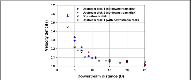
(11) Figure 4-8: 3D view of Chacao Channel bathymetry. (Herrera, 2010). .......................... 62 Figure 4-9: Chacao Channel Seagrid model grid of 82 rows and 143 columns. ............. 63 Figure 5-1: Tidal wave amplitude resonance from Guafo mouth to Reloncaví Sound. .. 67 Figure 5-2: Modeled flood flow velocities (m/s) at Syzygy. ........................................... 69 Figure 5-3: Modeled ebb flow velocities (m/s) at Syzygy. .............................................. 69 Figure 5-4: Modeled flood flow velocities (m/s) at Quadrature. ..................................... 70 Figure 5-5: Modeled flow velocities (m/s) at Syzygy. ..................................................... 70 Figure 5-6: Tidal velocities at Carelmapu (green) and Remolinos Rock (blue), compared with tidal differential between both sides (red)................................................................ 72 Figure 5-7: Zoom in to lag between peak tidal differential and peak velocities, in order to calculate response time due to drag. ............................................................................ 73 Figure 5-8: Portion of modeled area defined for profile analysis. (SHOA, Cartas y Publicaciones Náuticas (Publicación SHOA N° 3000), 2010). ....................................... 74 Figure 5-9: Mean depth (a) and width (b) along transversal profiles of the Chacao Channel. ........................................................................................................................... 74 Figure 5-10: Transect detail to calculate flows and power along the Channel. ............... 75 Figure 5-11: Velocity profile analysis along the Chacao Channel. ................................. 76 Figure 5-12: Power profile analysis along the Chacao Channel. ..................................... 76 Figure 5-13: Velocity in Y direction (perpendicular to flow direction) profile analysis along the Chacao Channel. ............................................................................................... 78 Figure 5-14: Maximum tide power (MW) in the Chacao Channel. ................................. 79 Figure 5-15: Mean tide power (MW) in the Chacao Channel. ........................................ 79 Figure 5-16: Chacao Channel bathymetry and equipment distribution division. (Winckler & Contreras, 2009).......................................................................................... 81 Figure 5-17: Areas of benthonic resources extraction. (Kosiel, 2012). ........................... 82 Figure 5-18: Areas of aqua farming activities. (Kosiel, 2012). ....................................... 83. x.

(12) RESUMEN La distribución del flujo de las mareas en el espacio y el tiempo es modelada y analizada en la región de los fiordos del sur de Chile y el Canal de Chacao, que une el Océano Pacífico y el Golfo de Ancud, separando la isla de Chiloé del continente en su lado norte. Las ondas mareales ingresan por el sur de la isla de Chiloé, presentando un comportamiento resonante en su viaje hacia el norte, con variaciones de hasta 6 metros en el Seno del Reloncavi. En consecuencia, las diferencias de altura de mareas significativas entre las entradas Este (Golfo de Ancud) y Oeste (Océano Pacífico) del Canal, producen velocidades de más de 3 [m/s] en algunos lugares de su extensión. De esta manera, este trabajo busca realizar una evaluación preliminar del recurso energético de las corrientes de marea para la extracción de energía renovable. El modelo Regional Ocean Modelling System (ROMS) se utilizó para crear un modelo regional 2D que reproduce el desplazamiento de la onda mareal alrededor de la isla de Chiloé, y a su vez genera condiciones de entrada para un modelo de mayor resolución del Canal. Las mareas modeladas en el modelo regional se validan (y calibran) con las mediciones de mareas existentes en cuatro puntos ubicados a lo largo del Canal (Manao, Tique, Pihuio y Carelmapu). El modelo regional tiene un tamaño de grilla de 5 kilómetros, adecuado para reproducir los fenómenos de marea en la región, y la grilla del Canal, un tamaño de 300 metros, lo que permite crear un mapa de alta resolución de las corrientes a lo largo del Canal, para el estudio de sus características y distribución. Las turbinas deben ser distribuidas adecuadamente y su cantidad limitada, para permitir la extracción óptima de energía a partir de un flujo de agua y mantener los impactos al mínimo. Este estudio describe el comportamiento de las mareas y los correspondientes flujos del Canal en 2D, con el objetivo de avanzar hacia la creación de un modelo 3D que incorpora la presencia de turbinas. Por último, se hacen sugerencias para la futura ubicación de equipos de medición, del proyecto de Investigación y Desarrollo en el que está enmarcado esta tesis.. Palabras Clave: marea, turbinas, recurso energético, modelo, ROMS, Canal de Chacao. xi.

(13) ABSTRACT Tidal flow distribution in space and time is modeled and analyzed for the southern fjords region of Chile and the Chacao Channel, one that joins the Pacific Ocean and the Ancud Gulf, and also separates the island of Chiloé from the continent on its northern side. Tidal waves enter south of Chiloé island and show a resonant behavior as they travel north, reaching tidal variations of around 6 meters in Reloncavi Sound. Consequently, the Chacao Channel has a significant tidal height difference between its eastern side (Ancud Gulf) and its western side (Pacific Ocean), which produce velocities of over 3 [m/s] at certain locations along its length. The latter motivates this work as a preliminary energetic resource assessment of tidal currents for renewable energy extraction. For the modeling process the Regional Ocean Modeling System (ROMS) is used to create a 2D regional model which reproduces tidal wave advance surrounding Chiloé Island, and creating input information for a nested 2D model of the Chacao Channel with finer resolution. Modeled tides in the regional model are validated with tidal measurements at four points located along the Channel (Manao, Tique, Pihuio, and Carelmapu), which allow a proper calibration of both models. The regional model has a grid size of 5 kilometers, enough to properly reproduce tidal phenomena in the region, and the Chacao Channel grid, a size of 300 meters, allowing creating a rather fine map of currents along the Channel as a way of studying it´s characteristics. Tidal turbines should be properly distributed and their amount limited, to permit the optimal energy extraction from a water flow and maintain impacts at its least. This study does a deep description of sea surface and 2D flow behaviors in the fjords region, and specifically the Chacao Channel, as a long run objective of advancing towards creating a future 3D model which incorporates the presence of turbines. Finally, suggestions for installation of measurement equipments in the R&D project are made, for future optimal model calibration.. Key Words: tide, turbines, energetic resource, Model, ROMS, Chacao Channel.. xii.

(14) 1. 1.. INTRODUCTION. This first chapter is an introduction to the context in which this thesis is developed. It also points out the main and specific objectives behind the investigation done, in order for the reader to understand the general structure and procedures followed through it. 1.1. Context. The raise in carbon emissions and oil prices, added to a coupled energy demand and country development rate, have forced researchers and developers to search for new sources of renewable energies. Although nowadays these energies present reasonably higher costs and lower plant factors than traditional energies (large hydroelectric dams and thermoelectric plants), it is only a matter of time before they become competitive. Wind power has undergone a rapid development; within the past years its global installed capacity has increased from approximately 2.5 GW in 1992 to a little below 40 GW at the end of 2003, with an annual growth rate of around 30% (Morthorst, 2004). In the same manner, Geothermal, Thermo Solar, Solar PV, Biomass, Wave and Tidal energies are all expected to decrease their costs, as their installed capacities (and experience) increases. Tidal energy exploits the natural ebb and flood of coastal tidal waters, caused principally by the interaction of the gravitational fields of the Earth, Moon and Sun. These tidal currents are magnified by topographical features, such as headlands, inlets and straits, or by the shape of the seabed when water is forced through narrow channels (Rosenfeld, Shulman, Cook, Paduan, & Shulman, 2009). In Chile, going south from the island of Chiloé, an abnormal geography composed by islands and channels or narrows is found, which is strongly marked by glacial action during previous ice ages (Borgel, 1970). These regions present a tremendous potential for the development of tidal energy, which could be used for small population energy supply, or even pumping energy to the main electric grids, in a few particular cases. One of these is the Chacao Channel, presenting currents around 3–5 [m/s], and categorized by Garrad Hassan Partners (an international consulting company with experience in the field of marine energy resource assessment).

(15) 2. as one of the best places worldwide for the development of a tidal farm (Garrad-Hassan, 2009). Based on these backgrounds, a public-private research and development project, entitled “Assessment of the Tidal Energy Resource in the Chacao Channel, for the Selection and Implementation of Energy Extracting Devices”, is being developed under the University’s management. One of the main products of the aforementioned project is to develop hydrodynamic models that should allow determining hot spots along the Channel, and the effect that a device or an array of devices may induce on the flow hydrodynamics. One of the potential outputs being to develop tools that support the efficient and optimal design of energy extraction farms. In order to advance in that item, this thesis searches to implement a gross (5 km grid) 2D regional model of the whole Southern Fjords and Chiloé region (also called Chilean Inland Sea) in ROMS, and nest a finer model (300 m grid) of the Chacao Channel in it. This way, a better resolution of the Chacao Channel is obtained, in order to comprehend the medium scale hydrodynamic processes that occur. Finally, recommendations of locations for tide gauges and ADCP’s are made, in order to obtain optimal input information for future models, which are a part of the aforementioned investigation project. 1.2. Objectives. Given that this thesis aims to advance in a specific area of the project afore mentioned, its objectives are linked with the objectives of that project. Therefore, the goals of this thesis are: Main Objectives: Implement a model that properly reproduces tidal travel through the northern Chilean Inland Sea, and nest a smaller one that estimates the energetic resource available in the Chacao Channel. Specific Objectives: Build and implement a 2D regional model of the complete southern fjords and Chiloé region of Chile, which can reproduce real tidal phenomena and.

(16) 3. therefore create good boundary conditions for a nested model. Study the tidal phenomenon existent in the Chilean Inland Sea (all around Chiloé Island), and particularly the resonance effect which causes large tide variations at Ancud Gulf and Reloncaví Sound. Create a hydrodynamic modeling tool with ROMS, which is applicable to Chacao Channel and nested in the larger scale regional model. Determine the space-time 2D flow distribution in Chacao Channel. Analyze results in the Channel as a 1D model, as an easy method of behavior analysis. Estimate potential energy that could be extracted and generated with tidal turbines in Chacao Channel. Recommend proper locations for tide gauges and ADCP’s, to obtain optimal real data generation, which allows good calibration of hydrodynamic models in Chacao Channel..

(17) 4. 2.. BASIC FUNDAMENTS AND REVISION. The first step was to carry out a detailed revision of the basic concepts involved in this thesis and papers and studies done to the date. Firstly an introductory revision of the main concepts behind tides and their operation will be revised and discussed, which will be based on information provided by the chapter on tides from the texts “Introduction to Coastal Processes & Geomorphology” by Masselink, G. and Hughes, M (2003), and “Tides, Surges and Mean Sea-Level” by Pugh, D. (1987). Once having explained the basic concepts behind tides, a revision of tidal models and tidal farms design will be addressed, in order to clear out for readers the status of investigation in the area. Finally, this chapter will close with a brief explanation of the area of study, together with a revision of main studies done up until now, which support the need for this specific thesis. 2.1. Tides. 2.1.1 Basic Concepts and Astronomic Forcing Tides are an effect of the gravitational force the Moon and Sun have over the Earth, which cause a rise and fall of the oceanic surface. This variation of the ocean´s surface is only noticeable in regions where it takes contact with land, along coastlines or shallow continental shelves, because in the open ocean its effect is very mild. The basis to tidal existence is explained by Newton´s law of universal gravitation which states that “every particle in the Universe attracts every other particle with a force that is directly proportional to the product of their masses and inversely proportional to the square of the distance between them” (Serway & Jewett, 2010), and is resumed in equation (2.1). This way, all planets in the Universe have some kind of gravitational effect over the Earth, yet they are insignificant in comparison to the Moon and Sun, because of their size or distance (Masselink & Hughes, 2003). (2.1).

(18) 5. Where G is the universal gravitation constant, m is the mass of the two bodies interacting, and R is the distance between the centers of mass of them. The Moon and Sun are the main tidal drivers, given their close proximity to the Earth and large size, respectively. It is their relative positions that determine the advance of tidal waves around the globe. First, the Earth rotates over its own axis in around 23.93 hours, which is called a solar day. At the same time, the Earth and Moon form a system that rotates anticlockwise around their common centre of mass or also called barycenter (located inside the Earth). One rotation of this paired system takes around 27.32 days, which is called a sidereal month. Finally, the Earth-Moon system barycenter rotates around the Sun, in approximately 365.24 days, called a year (Masselink & Hughes, 2003). The tidal waves are formed by the interaction of two main forces, centripetal and gravitational, that give place to the tide generating force. The first provides the acceleration every particle of mass on the Earth requires to maintain its orbital motion, and particularly to maintain the Earth-Moon system rotating in a stable manner. It is resumed in equation (2.2), it does not depend on location on the Earth's surface, and its direction is always parallel to the plane of rotation of the Earth-Moon system. The second, the local gravitational force, depends on location and is given by equation (2.3). This way, on the Moon facing side of the Earth the gravitational force will be larger than the force experienced on the opposing side. The average centripetal force per unit of mass must equal the average gravitational force per unit of mass, in order to maintain the rotation of the Earth-Moon system stable. Otherwise, they would accelerate towards each other (Masselink & Hughes, 2003). (2.2) (2.3) Where r is the distance between the Earth’s center and the point of interest on the Earth’s surface, mE is the mass of the Earth, and mM is the mass of the Moon..

(19) 6. A small acceleration is experienced in different locations of the Earth, due to the local gravitational force differences, which is applied and observed over the ocean mass. This way, the vector resultant from the addition of both forces is called the tide-generating force, which causes these local accelerations, and is expressed in equation (2.4). It will be positive on the Moon facing side (towards), and negative on the opposing side (away from). Finally, the Ocean surface is drawn towards two points at opposing sides of the Earth (Masselink & Hughes, 2003). (2.4) Although one might tend to think that the local variation of this force causes the ocean water on the Earth’s surface to be drawn towards opposite sides of it, this ignores that this force is very small compared to the Earth’s own attractive force acting upon the ocean and directed to its centre at every point. Therefore, it is actually the vector component of the tide-generating force, which is tangential to the Earth’s surface that draws the ocean into two bulges on either side. This tangential component of the tidegenerating force is known as the tractive force, and is shown in equation (2.5) (Masselink & Hughes, 2003) (2.5) In this case, θ is the angle between the point of interest on the Earth’s surface and the line joining the centers of the Earth and Moon. Finally, one can observe how the phenomena explained works in reality, and the effect these have over the Earth surface. It is seen how bulges at both sides of the Earth are formed, and how the forces applied over it affect the tide propagation. Figure 2-1 summarizes the interactions explained recently..

(20) 7. Figure 2-1: Tidal astronomical forcing interaction.1 2.1.2 Tidal Reference Levels Tides are a variation of the level of the sea, which makes it extremely important to understand how these levels are measured and the references that are used in Chile to define their variation. Figure 2-2 sketches the different tidal levels considered.. 1. University of Victoria, http://web.uvic.ca/~rdewey/eos110/webimages.html..

(21) 8. Figure 2-2: Main tidal reference levels, according to Chilean Navy rules. (SHOA, Glosario de Mareas y Corrientes (Publicación SHOA N° 3013), 1992) Previous to mentioning the different reference levels, concepts of low and high tide must be defined: -. High Tide: Maximum sea level attained by a flood tide (increasing sea level or tidal wave travelling from open sea towards land). This can be caused either exclusively by periodic astronomic tides, or meteorological conditions could also be involved (SHOA, Glosario de Mareas y Corrientes (Publicación SHOA N° 3013), 1992).. -. Low tide: Minimum sea level attained by an ebb tide (decreasing sea level or tidal wave travelling from land towards open sea) (SHOA, Glosario de Mareas y Corrientes (Publicación SHOA N° 3013), 1992)..

(22) 9. Reference levels adopted in Chile and sketched in the last figure are explained next (SHOA, Instrucciones Oceanográficas N° 2, Método Oficial para el Cálculo de los Valores No Armónicos de la Marea (Publicación SHOA N° 3202), 1999): -. Mean Tidal Level: equidistant plane between mean high tides and mean low tides, for a long period of observations.. -. Mean Sea Level (M.S.L.): it corresponds to the mean level of sea level movements, which would be equivalent to the level sea would have is tides did not exist. To obtain this level, all hourly data of an observation period must be averaged.. -. Mean Level of High Tide: is equivalent to the average of all high tides registered during the observation period.. -. Mean Level of the highest High Tide: given Chile’s geographical location, both high tides seen in a day, have a significant height difference. Therefore the daily highest high tide is defined as so, and all highest high tides of an observation period are then averaged to obtain this level.. -. Mean Level of Low Tide: is equivalent to the average of all low tides registered during the observation period.. -. Mean Level of the lowest Low Tide: as for high tides, low tides in Chile also present two peaks with different levels in a day. Therefore the daily lowest low tide is defined as so, and all lowest low tides of an observation period are then averaged to obtain this level.. -. Probe Reduction Level (P.R.L.): it is the plane for which probes or depths are referred to at a certain location. Navigational necessities require that nautical charts show the lowest depth able to be found at a certain point; therefore usually probes in a chart are referred to some level related to low tides.. 2.1.3 The Equilibrium Theory of Tides The equilibrium theory of tides has three main assumptions (Pugh, 1987):.

(23) 10. i). The Earth is covered entirely by an ocean of uniform depth, meaning there are no continental land masses.. ii). There is no inertia in the system, meaning the oceans respond immediately to the tide-generating force.. iii). The Coriolis and friction effects can be neglected.. Basically this theory assumes that under the lack inertia in the system, the tidal bulges will follow the Moon around the Earth. Figure 2-3 shows the comparative position of both bulges with respect to lunar position, at different moments of the month.. Figure 2-3: Solar-Lunar interaction as a tidal generator.2 As mentioned before, not only does the Earth and Moon rotate together around their barycenter, also the Earth spins in an anticlockwise direction on the axis that goes through its poles in 24 hours. Therefore an observer at a certain point will experience two high tides and two low tides in a day or complete spin of the Earth. At the same time, the Moon also rotates around the Earth, and advances 12.2 degrees per day, therefore shifting the tidal bulges by the same amount every day. This explains the variation of tidal peaks from one day to another.. 2. http://mail.colonial.net/~hkaiter/Moon_Phases_Tides.html..

(24) 11. The assumption used up until now, where Moon is aligned with the Earth’s equator, is actually not completely real and produces certain changes over the system. In reality the Earth-Moon system is tilted by angle of approximately 28.5°with respect to the Earth’s equatorial plane, also known as the lunar declination. This means that tidal bulges formed around the Earth are also tilted with respect to the equatorial plane. This means that an observer located at a certain point above or below the Equator will experience a daily variation between both high tides and low tides. The largest daily variation will occur when at the times in the month when the Moon is positioned over the tropics, called tropical tides. On the contrary, the smallest daily variation (or null variation) will occur at the times in the month when the Moon is positioned above the Equator, called equatorial tides. Both of these usually occur twice a month (Pugh, 1987). Not only does the Moon produce a tide-generating force over the Earth, the Sun has the exact same effect yet a 46 % of that produced by the Moon. This difference is due to the closer proximity of the Moon to Earth, and even though the Sun’s mass is much larger, it is not enough to compensate for distance. The presence of the Sun is traduced in a moderating or amplifying effect of tides, which depends on its relative position with the Moon and Earth. When the Moon is new or full the Earth, Moon and Sun are aligned, so are their bulges, which yield tidal bulges that are the sum of the individual contributors. This moment of the month is called syzygy. On the other hand, when the Moon is in at a right-angle to the Earth with respect to the Sun, so are their bulges, which yield tidal bulges that constructively interfere with each other. This moment of the month is called quadrature. In summary, tides during syzygy are largest and are called spring tides, whereas tides during quadrature are smallest and are called neap tides. Each occurs approximately every 15 days (Pugh, 1987). The Moon and Sun orbit shapes also have an effect over tides. Until now, circular paths were considered, yet in reality paths are elliptical, which means distances between bodies differ at different moments of the path. The Moon is closest to the Earth at perigee (357,000 km), and furthest at apogee (407,000 km), meaning tide-generating force will be larger at perigee than apogee. As a result, one of the spring-neap tides in a.

(25) 12. given month is larger than the other. As well, there will be an occasion when the new moon coincides with perigee and one when full moon does so, usually March and September. In the same way, the orbit of the Earth-Moon system is also elliptical, therefore the Sun is closest to the Earth at perihelion (148,500,000 km), and furthest at aphelion (152,200,000 km), producing a stronger effect over tides at perihelion. Thus the tides are marginally larger in the 6 months centered on January, and marginally smaller in those centered on July (Pugh, 1987). Finally, the Sun’s position over the Earth varies between the Tropic of Cancer (latitude 23.5°North) and the Tropic of Capricorn (latitude 23.5°South), and back again in the course of a year or 365.25 days. When it is over the tropics, during solstices, the solar tidal bulge will add a small amount to the diurnal inequalities in tide range produced by the lunar declination; whereas over the Equator, during equinoxes, it will not. In the long run, there is a precession of the lunar declination with respect to the solar declination, which produces an 18.6 year periodicity in the tides (Pugh, 1987). Figure 2-4 shows the contribution of some components to the time series at Longyearbyen, allowing clear understanding of the dynamics of tidal time series (Gjevik, 2006). Even though it seems as if this theory can explain most of the observed features of tides, there are four shortcomings (Masselink & Hughes, 2003): i). The predicted tide range is typically smaller than the observed range.. ii). The predicted tidal range is not constant, but varies with location around the globe.. iii). The timing of high water is generally several hours before or after the time of transit of the Sun and Moon.. iv). The timing of spring and neap tides does not always coincide with syzygy or quadrature, but is typically a day or more different.. These make one conclude that there is some sort of preferential response to the tide generating force, determined by local characteristics, and assumptions of zero inertia and friction are too restrictive. This is why Equilibrium Theory cannot be used in any precise way to predict the tide at a given location..

(26) 13. Figure 2-4: Tides at Longyearbyen 1-31 October 2006. a) Only M2, b) M2+S2, c) M2+S2+N2, d) M2+S2+N2+K1. Full Moon 7 Oct., New Moon 22 Oct. Lunar perigee 6 Oct. and apogee 19 Oct. Day starts at midnight UT (GMT). (Gjevik, 2006)..

(27) 14. 2.1.4 The Dynamic Theory of Tides Given that the Equilibrium Theory does not explain real tides on its own, due to the basic assumptions that characterize it, the Dynamic Theory of tides was developed by contributions made by Bernoulli (1740) and Laplace (1775) (Gjevik, 2006). In it, the basic assumption is that the two tidal bulges discussed before behave as waves, and because of their extensive wavelength (compared to water depth), they specifically are considered to behave as long waves or shallow-water waves. Therefore a long wave is associated to every tide-generating force contributor (Moon and Sun), and as they are always present the long wave is always being driven by it. These waves are called forced waves. The limited ocean depth, which restricts long wave velocity, and the fact that the ocean is not continuous, but separated into several deep basins, traduces in long waves effectively being broken up into smaller systems. These systems are called amphidromes, and they work in such a manner that long waves rotate around a central point where tidal variation is null. The amphidromic systems along the Earth are shown in Figure 2-5, and as can be noticed, the sense of rotation is clockwise in the Southern Hemisphere and anticlockwise in the Northern Hemisphere. This way, Earth rotation and Coriolis Effect produce a wave crest (and opposite trough) rotating around an ocean basin, in the senses mentioned for each Hemisphere, and these waves are called Kelvin waves (Pugh, 1987)..

(28) 15. Figure 2-5: World tidal patterns and the amphidromic points.3 2.1.5 Tidal Level Prediction As has been explained up until now, tides are consistent phenomena, which depend on astronomical cycles, and therefore are extremely predictable. In order to predict tides at a specific location there are several methodologies, yet the main one is called the Harmonic Analysis method. This is a method by which an observed tide can be modeled as a sum of a certain number of harmonic constituents or partial tides, which periods correspond to the periods of some relative astronomical movement between the Earth, Moon and Sun. The partial tides are harmonics the periodic motion of the water surface elevation at one location is expressed in terms of a cosine function that includes time. Equation (2.6) shows how the reconstruction of the observed tides is done (Masselink & Hughes, 2003). (2.6) Where. is the tidal water level, t is time,. is the mean sea level, and a i , f i and G i. are the amplitude, frequency and phase of the i-th partial tide, respectively. The last term 3. Modified from R. Ray, “TOPEX/Poseidon: Revealing Hidden Tidal Energy”, GSFC, NASA..

(29) 16. r. is the residual water level, which is a correction term for differences between. predicted and observed tidal records. At different locations, each partial tide has a specific amplitude and phase, which depend on the geographical conditions of that place. Therefore, tidal prediction by the method of harmonic analysis typically involves a least-squares fitting of the principal partial tides to an existing tidal record for that location, in order to obtain their amplitudes and phases. Length of data series will determine the amount of constituents to be considered in the analysis, therefore longer series implies more constituents. This follows the Raleigh criterion for statistical analysis. Finally amplitudes, frequencies and phases obtained are then replaced in equation (2.6) to predict tides in the future (Masselink & Hughes, 2003). 2.1.6 Tidal Classification Tides at different locations are rated depending on the local predominant tidal regime, which is defined using the criteria of the Courtier coefficient (SHOA, Glosario de Mareas y Corrientes (Publicación SHOA N° 3013), 1992). This coefficient is obtained from an amplitude relationship of the main semi diurnal and diurnal tidal harmonic constituents, calculated using equation (2.7). (2.7) Where the parameters are the amplitudes of each tidal constituent: a K 1 = Lunar-solar declination diurnal component.. aO1 = Lunar declination diurnal component. a M 2 = Main lunar semi diurnal component.. a K 1 = Main solar semi diurnal component.. Finally, replacing these parameters in the equation, a value for the coefficient is obtained, which described the characteristic of tidal regime at that certain spot. The ranges for the values obtained are rated as follows:.

(30) 17. F < 0.25 0.25 < F < 1.50. Mixed regime, predominantly semi diurnal tide.. 1.50 < F < 3.00. Mixed regime, predominantly diurnal tide.. F > 3.00 2.2. Semi diurnal tide regime.. Diurnal tide regime.. Tidal Energetic Flow Models. As explained before, tidal waves are extremely predictable, due to the fact that they are driven by predictable astronomical motions. Therefore tidal models are a rather precise tool, and very useful to explain their local phenomena’s in coastal regions. Many tidal models have already been developed, with different purposes of course: sediment transport, inter tidal biodiversity, energetic resource, among others. Regarding the evaluation of tidal flow energetic resources in fjords or channels, estimations are based on the use of basic hydrodynamic equations, for one dimension, two dimensions or three dimensions: momentum balance and continuity. Basically studies developed up until now are separated into three main branches, depending on their scale: -. Tidal Energetic Resource (Large scale): Consists in models in which tidal flows and energetic potential are modeled, and the presence of turbines is incorporated to the basic equations, in order to determine their general effect as an extra drag coefficient.. -. Tidal Farm Design (Medium Scale): Tidal flows are modeled with the presence of tidal farms, yet in this case flows are analyzed at smaller scale, in order to define distance between turbines in a row and between rows of turbines. This aims towards designing an optimal array of tidal turbines.. -. Flow-Turbine Interaction (Small Scale): The interaction between turbine blades and flows are modeled and analyzed, in order to develop and define the adequate turbines to be used for a specific location..

(31) 18. All three branches are related, and must be incorporated into the large-scale tidal flow model, when one decides to design a definitive tidal farm. In these case studies related to the large and medium scale will be mentioned and analyzed, in order to introduce the actual status of research relating tidal models. Small-scale studies are beyond the scope of this particular thesis, given that the analysis of specific types of turbines is being tackled by other students in the framework of the Research & Development project. 2.2.1 Tidal Energetic Resource a). Main Concepts. As has been studied for turbine array distributions in wind farms, the effect of a turbine over the fluid’s natural flows must be considered in the modeling process, in order to ensure an optimal extraction of energy and therefore of farm design. At first, energetic potential in wind flows was estimated by the kinetic energy (KE) available in a certain transversal area of the flow, which is shown in equation (2.8) (Garret & Cummins, 2005). (2.8) Where ρ is the fluid’s density, A is the area spanned by the turbine, and u is the velocity of the flow. In 1927, Betz discussed a simple model, in which he estimated that the maximum power attainable (MPA) was 16/27, or 59%, of the kinetic energy available in a flow, before it passes through the section of a turbine (given in equation (2.9)) (Betz, 1926). Although, Bergey (1980) argues it was earlier derived by Lanchester (1915). This limit to maximum power is called the Lanchester-Betz limit (Bergey, 1980). Some investigators believe this is unrealistic, due to the several assumptions Betz made to attain this value. As a matter a fact Gorban et al. (2001) obtained that, if curvature of streamlines were allowed, the efficiency factor drops down to 35% (Gorban, Gorlov, & Silantyev, 2001). (2.9).

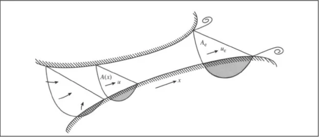
(32) 19. The large scale and small scale flow-device interaction has been widely studied for the case of wind farms, but not that much for tidal farms, yet the basic concepts of the first are applicable to the last. Some investigators have already begun to study the tidal flow energetic resource, and ways of incorporating the effect in a 1D, 2D or 3D model of a certain channel or fjord. Basically, the effect of turbines over hydrodynamic flows is incorporated into models as a sink of momentum, present as an additional drag coefficient in the basic flow equations (Blanchfield, Garrett, Wild, & Rowe, 2008). This way, Garrett and Cummins (2005) determined that kinetic energy overestimates the energetic potential of a channel, given that it does not take into account the influence turbines have over flows. A 1D model developed by them demonstrated how the incorporation of turbines into a channel, increased the total drag, therefore slowing down the hydrodynamic flows. This model considered flow through a channel of variable cross-section (as shown in Figure 2-6), and with dynamic equation (2.10) governing the flow’s momentum budget (Garret & Cummins, 2005). (2.10) Current speed u ( x, t ) is assumed to vary with time t and position x along the channel. The slope of the surface elevation. provides the pressure gradient to drive the flow, and. F ( x, t ) represents an opposing force related to natural friction along the channel and the incorporation of turbines. Finally, if the channel is short compared to the tidal wavelength (which will usually be so, unless the channel is extremely long), volume conservation implies that the flux Au along the channel is independent of x and may be written as Q (t ) ..

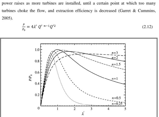
(33) 20. Figure 2-6: Channel of variable cross-section, which connects two basins with different tidal elevations. (Garret & Cummins, 2005). By solving the basic equations, the authors managed to develop a model, which can give good preliminary estimates of power potential at different sites worldwide, obviously considering modifications for specific local characteristics. The main result obtained was that, to within 10%, the maximum average power available is approximately. 0.22 gaQmax , for a sinusoidal tidal head a cos t and with Qmax denoting the peak volume flux in the undisturbed state (Garret & Cummins, 2005). Another important result came from realizing that F (friction due to turbines) integrated along the channel, gives equation (2.11), in which Q is the flow and λ is related to the number of turbines and their position along the channel. This is extremely important, because it represents one possibility of representing small-scale turbine and farm effects into a large-scale model. Therefore, in farm design it is important to assess the overall effect of turbines by a single parametric coefficient (Garret & Cummins, 2005). (2.11) Finally, an exponential turbine drag in the current speed ( Q. n 1. Q ) is used to estimate. the extractable power to a more realistic degree. Including this hypothesis in the basic hydrodynamic equations, non-dimensional equation (2.12) is obtained and then drawn.

(34) 21. for different values of n in Figure 2-7. This way it is clearly observed how extracted power raises as more turbines are installed, until a certain point at which too many turbines choke the flow, and extraction efficiency is decreased (Garret & Cummins, 2005). (2.12). Figure 2-7: Power extraction as a function of the nth exponential and nondimensional turbine drag (λ). (Garrett & Cummins, 2007). The study of Garrett and Cummins (2005) sets a base to a series of following studies, which is why it was important to explain in depth the procedures followed and the conclusions obtained. More advanced studies search to model flows in channels, applied to: specific locations (Defne, Haas, & Fritz, 2011; Rosenfeld, Shulman, Cook, Paduan, & Shulman, 2009); considering different topographical aspects and configurations (Blanchfield, Garrett, Wild, & Rowe, 2008); impacts on different hydrodynamic aspects (Polagye, Malte, Kawase, & Durran, 2008); and, varying turbine concentrations and distributions (Garrett & Cummins, 2008)..

(35) 22. Important points to recall from these papers are methodologies followed and the results obtained, in order to use them understand the structure and concepts behind tidal models, and as a basis for this and future studies in Chacao Channel. b). Real Applications. Not only is it important to revise the physical procedure used to model channels, but also think about the possible “products” which one searches to develop and the methodologies used. There are a series of studies relating hydrodynamic modeling (using ROMS, Mike 21, among others) at different spots around the world, and it was interesting to use their procedures as guides. Rosenfeld et al (2009) and Defne et al (20010) modeled tides and currents with ROMS, and following a procedure very similar to the one proposed here. Investigations are based on 2D and 3D models, which are either fed with inputs from measurements or calibrated with them, which is done by comparing tidal components amplitudes at specific locations and other statistical parameters (Defne, Haas, & Fritz, 2011). Once having calibrated, results regarding tidal velocities at attractive locations, including tidal ellipse figures and maps with power density along the spots, as can be seen in Figure 2-8..

(36) 23. Figure 2-8: Mean power density maps along (a) the northern and (b) the southern coasts of Georgia with labeled high tidal streampower density (>500 W/m) areas. (Defne, Haas, & Fritz, 2011) Finally, these studies help to guide the procedures and results to be presented in this study, in order to assure a proper “product” that can be used in future studies, and therefore is of value towards the design of a future tidal farm. 2.2.2 Tidal Farm Design The past section detailed studies relating large scale models of a 1D flow in a channel and the effect that turbines induce over it, this section refers to a smaller scale, and revises studies regarding the optimal design of tidal farms and turbine spacing. Several investigators have addressed these issues and have explored them to a laboratory scale,.

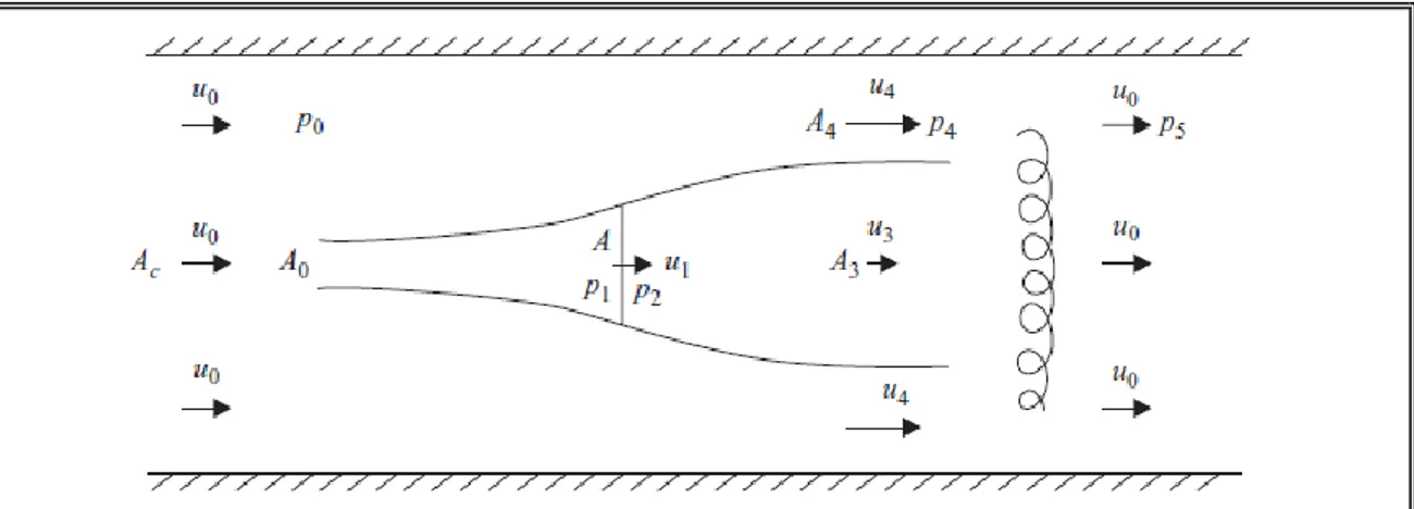
(37) 24. in order to understand turbine interactions and optimal spacing between devices, for future real scale tidal farm designs. This is a concept that began many years ago with wind farm research, when the first wind turbine arrangements had to be considered (Betz, 1926). These issues started off with the Lanchester-Betz limit, also mentioned in the past section, given that it sets a maximum extractable energy from a certain available energy in a flowing fluid (Bergey, 1980). From there, Garrett and Cummins concluded in 2007, that optimal tidal farms involved occupying a complete transversal section of a channel. This conclusion came from the fact that gaps between turbines produced downstream mixing of enhanced flows through these gaps and slower flows passing through turbines, which bring energy dissipation (as seen in Figure 2-9). Therefore, tidal design must search to span the largest portion of the channel’s section as possible (Garrett & Cummins, 2007).. Figure 2-9: Definition sketch for a single turbine in a channel (Garrett & Cummins, 2007). In the mentioned paper, the fraction u 3 / u 0 is brought up as a tuning parameter to optimize energy extraction from hydrodynamic flows, being its ideal value 1/3. Therefore, it is concluded that maximum energy produced by the turbines is a fraction of the potential of a complete tidal fence (row of turbines spanned perpendicular to the flow direction), with the fraction being 2/3 if they occupy a small fraction of the channel.

(38) 25. cross-section and decreasing to 1/3 if occupying most of the section. Quantitatively, an optimal number N of partial fences is expected to be calculated with equation (2.13) (Garrett & Cummins, 2007). (2.13) Where each parameter is: ε: Fraction of the cross-sectional area taken up by the turbines.. AC : Cross-sectional area. u 0 : Turbine upstream flow velocity. P: Power generated by the turbines. In 2010, Vennell also concluded that to maximize turbine efficiency with a minimum number of turbines, the configuration must be designed to occupy the largest crosssectional area permitted by navigational and environmental constraints. Maximum energy production requires the turbine blades to be tuned for a particular channel and turbine density, which is influenced by its drag coefficient, length, width and depth, tidal frequency and amplitude. This leads to the need to tune blade pitch in real time along a tidal cycle to maintain the u 3 / u 0 parameter at a constant optimal value. Therefore farms should first add turbines to its rows, and then add new rows if necessary. This is shown in Figure 2-10, as power is remained when cross-sectional area is optimized over row number (Vennell, 2010)..

(39) 26. Figure 2-10: Tuning and power at optimal tuning for an inertial channel, 0. 0 . (a) Optimal tuning, r3opt ( , N R* ) . (b) Fraction of a channel’s potential available for production, P avail / P max . (Vennell, 2010).. These results refer to the general rules one must consider when designing a tidal farm, yet several other studies enter in the detail of lateral and downstream distances between turbines which should be used for optimal turbine efficiency. In 2010, Lee et al modeled the tidal farm shown in Figure 2-11, where a lateral distance of two turbine diameters (. D S ) was considered, in order to determine an optimal downstream distance between rows. Results presented in Figure 2-12, demonstrate that an optimal efficiency is obtained at a downstream distance of three diameters, and remains constant at larger values (Lee, Jang, Lee, & Hur, 2010)..

(40) 27. Figure 2-11: Tidal farm model. (Lee, Jang, Lee, & Hur, 2010).. Figure 2-12: Results of tidal farm model, which show how at a downstream distance of 3D optimal turbine efficiency is obtained. (Lee, Jang, Lee, & Hur, 2010). Another similar study by Myers & Bahaj this year (2012) modeled a farm of turbines and validated it with laboratory scale measurements. Porous disks were installed in a laboratory channel to reproduce tidal turbines in a real scale channel, and different.

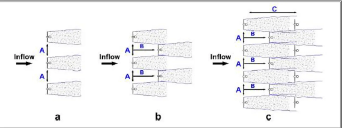
(41) 28. arrangements were evaluated in order to advance towards an optimal design. Figure 2-13 shows the dimensions of distances analyzed in the arrangements.. Figure 2-13: Arrangements of turbines in a channel and the dimensions studied to study their efficiency. (Myers & Bahaj, 2012). Figure 2-14 shows the results for a dual single row arrangement of turbines, where one can observe how extremely close turbines produce a combined wake (a), that has further downstream velocity deficit (percentage loss of undisturbed velocity) effect than single wakes as turbines are separated by a larger distance (b and c) (Myers & Bahaj, 2012). Therefore, one conclusion was that when designing an array, one must determine a minimum lateral distance which avoids this effect..

(42) 29. Figure 2-14: Model results of a dual single row arrangement of turbines over velocity deficit. (Myers & Bahaj, 2012). Finally, Figure 2-15 sketches the velocity deficit effects of a two row arrangement, where an inferior level of velocity deficit is obtained at approximately 10 to 15 diameters, which is a larger result than that obtained by Lee et al. Another conclusion reached was that a third row of devices could be installed far downstream, but in a shortmedium term wider 2-row arrays would offer a more favorable arrangement for a fixed number of devices within an array (Myers & Bahaj, 2012)..

(43) 30. Figure 2-15: Longitudinal centerline velocity deficits for the two row turbine arrangement. (Myers & Bahaj, 2012). All the results presented in this section allow understanding the stage at which tidal farm modeling and design are at present. This establishes the basic concepts and ideas that must be followed when a future tidal designing a farm that would be incorporated in the hydrodynamic model considered in this thesis. Once the proper procedure to incorporate their effect over tidal flows is defined, a tidal farm design must be thought of in terms of installed capacity, and therefore amount of turbines. Having a clear idea of how one must arrange them in a certain space, to extract as much energy as possible, will be extremely important for the incorporation in the tidal model. 2.3. Chacao Channel and the Southern Fjords. This section aims at establishing the basis of existent studies and data in the Chacao Channel and fjords region, so that results and conclusions obtained in this thesis improve those already suggested by previous studies. As well, knowledge of available data will allow deciding what data is useful and what data is missing for the models to be developed next..

(44) 31. 2.3.1 Existent studies and papers The southern coast of Chile, surrounding the great island of Chiloé, made up by a complex of channels and fjords, has caught the attention of fisherman, navigators, investigators, among other stakeholders, for a long time. Tides play an important role in several aspects of the region, including sediment transport, mixture and hydrodynamic current formations (García & Winckler, 2009; Salinas & Hormazábal, 2004; Silva, Calvete, & Sievers, 1997). This last point has brought to consider energy extraction from these currents for local, and even national, supply. In particular, Chacao Channel has been the main attraction, given its consistent fast flows, moderate depths and proximity to the Central Interconnected System (main Chilean electric grid). An international consulting company has identified Chacao Channel as one of the best spots in the world for the installation of tidal energy extraction devices, with a raw energy estimated between 600 and 800 MW, of which approximately 20 - 60% should be technically extractable, depending on spatial variation of the flow, bathymetry, and navigation requirements (Garrad-Hassan, 2009). Figure 2-16 shows three major channels with energy extraction potential, from which Chacao Channel is by far the most attractive.. Figure 2-16: Characteristics of three top energetic tidal channels in Chile, where Chacao Channel is by far the most attractive alternative. (Garrad-Hassan, 2009)..

(45) 32. This region, also known as the Chilean Inland Sea (CIS), is divided in two main areas: the northern and southern CIS, as seen in Figure 2-17. Both have their own geographical characteristics, and therefore behave different with tidal wave propagation, yet are correlated between each other (Aiken, 2008). The main ocean water entrance, called Guafo Mouth, is the boundary between both areas, and allows an interaction. The northern (nCIS) side is made up by Chiloé Island, Chacao Channel, the Gulfs of Ancud and Corcovado, and has a larger area of water for tidal waves to travel. Instead, the southern side (sCIS) is rather different, in the sense that it is composed by several small channels, fjords and islands, which give tidal propagation (therefore hydrodynamic models) a harder job, although it is more exposed to open ocean. This side begins at Guafo Mouth, is composed by its main Moraleda Channel, and ends at Elefantes Estuary.. Figure 2-17: Detailed map of the CIS, including a description of main channels and gulfs. (Aiken, 2008)..

(46) 33. Main scientific studies began to appear 10 to 15 years ago, and aimed at explaining the tidal wave propagation and related phenomena in the whole southern fjords region. In 2003, Cáceres et al studied tidal phenomena in the region, and analyzed the amplitude differences at certain points around the CIS, concluding that resonant conditions in the nCIS might exist (Cáceres, Valle-Levinson, & Atkinson, 2003). The existence of tidal variations of around 6 m at the Gulf of Ancud (Channel’s east side) and 2 m at Coronados Gulf (Channel’s west side), produce a head difference at either side of the it, which is traduced in flow velocities from 3 to 4.5 m/s in the Chacao Channel (Cáceres, Valle-Levinson, & Atkinson, 2003). A diagram showing this effect is presented in Figure 2-18, where it is seen how sea level difference causes a flow of water masses.. Figure 2-18: Diagram of tide level differences between both sides of Chacao Channel. A later study done by Aiken in 2008, further emphasized the existence of tidal resonance of waves propagating northward along the Gulfs of Corcovado and Ancud, and actually proved it analyzing several variables. Figure 2-19 sketches tidal wave amplitude from Guafo Mouth to Reloncavi Sound, showing how the tidal wave length resonates along the Northern CIS, increasing its amplitude and also changing its phase. The resonant frequency is a bit larger than semi diurnal components, being close to 10h 2008).. 1. ( (Aiken,.

(47) 34. Figure 2-19: Amplitude (upper) and phase (lower) of a damped channel harmonically forced at its open end. The dashed curves indicate the modeled amplitude of M2 in the nCIS. For the solid curves, r/ω= 0.3. (Aiken, 2008). Another interesting conclusion that was reached by Cáceres et al. (2003), was the flow pattern of the transect where Remolinos Rock is located, where the influence of lateral variations of bathymetry produce recirculation around the pinnacle and over the slopes of the Channel. There, mean flow is flood dominated at all depths in shallow areas, and ebb dominated in the deeper areas of the same cross section. This way, recirculation reflects strong divergences and lateral shears that translate into a relevant contribution of nonlinear terms (advection, horizontal and vertical friction) to the momentum balance (Cáceres, Valle-Levinson, & Atkinson, 2003). This can be observed in Figure 2-20, as the arrows show in and out flow in different areas of the same cross section, and can be an important aspect to analyze at different sections of the Channel, in order to identify precisely the flow patterns for farm design..

(48) 35. Figure 2-20: Schematic representation of the along-channel mean flow at Remolinos Rock transect. Outflow (gray arrows) and inflow (black arrows) regions are separated by strong convergences or lateral shears represented by the dashed lines. (Cáceres, Valle-Levinson, & Atkinson, 2003). The conclusions and results obtained by these studies set the base for this particular thesis, which is in line with other investigations carried out at other tidal channels, aims at characterizing important aspects and conclusions related to tidal phenomena and energy resource assessment in the CIS, and especially in the Chacao Channel. A few other public studies and thesis relating the same area have been released in the past years, yet their results add no new information which is relevant to this thesis. 2.3.2 Available Data in the Channel Last section was a brief compilation of main public studies that have been done in Chacao Channel and the fjords region. Additionally, a cadastre of available data in the region and Channel is also extremely important, in order to use those which are of proper quality and characteristics for the model built in this thesis, and further propose data collection locations for inputs in future models..

(49) 36. Data required for models in this case are basically three: bathymetry, sea surface levels (tides), and flow velocities. a). Bathymetry. Bathymetry in these two models is taken from digital versions of Nautical Charts, given by SHOA. Figure 2-21 shows the Nautical Chart 7210, which is for the Chacao Channel, and also points out the locations of available tides (red) and flow velocities (blue) data. There are also nautical charts of a larger scale for the whole fjords region.. Figure 2-21: Available current and tide measurements in Chacao Channel. (Herrera, 2010). b). Tides. Regarding tide measurements (or sea surface levels), there is available data at five points, which are detailed in Table 2-1, and their location specified in Figure 2-21. This data is a combination of SHOA measurements, and some measurements contracted by the Chilean Ministry of Public Works for a preliminary evaluation of a bridge that crosses the Chacao Channel (ICUATRO-COWI, 2000). These were not taken thought.

(50) 37. for model inputs, therefore there quality is not the ideal for the purposes required in this study, yet they are good enough for an initial modeling approach. Table 2-1: Summary of available tidal height measurements in modeled area. (Herrera, 2010). Station. Latitud. Longitud. Measurement. Period Considered. Manao. 41° 51' S. 073° 30' W. 41 days. 03/12/1999 - 12/01/2000. Tique. 41° 48' S. 073° 24' W. 106 days. 30/11/1999 - 14/01/2000. 05 days. 04/07/2000 - 08/07/2000. 46 days. 23/07/2000 - 06/09/2000. Eje - 1. 41° 48' S. 073° 32' W. Permanent. 03/12/1999 - 24/01/2001. Carelmapu. 41° 45' S. 073° 43' W. Permanent. 15/01/2000 - 22/01/2001. Pihuio. 41° 49' S. 073° 41' W. 36 days. 26/05/2000 - 30/06/2000. c). Flow Velocities. Finally, flow velocities in the Channel are available at three specific points, which are detailed in Table 2-2, and once again their location specified in Figure 2-21. Table 2-2: Summary of available velocity measurements in modeled area. (Herrera, 2010). Station. Latitude. Longitude. Measurement. Period. Roca Remolinos. 41° 47' S. 072° 32' W. 57 days. 11/07/2000 - 05/09/2000. Puerto Elvira. 41° 47' S. 073° 35' W. 56 days - 1 hour. 12/07/2000 - 05/09/2000. Bajo Seluian. 41° 48' S. 073° 31' W. 57 days - 1 hour. 11/07/2000 - 05/09/2000. At Roca Remolinos, the ADCP was installed at 28 meters depth, using nine sampling layers of 2 meters thickness each. Measurements were done between depths 3.21 to 21.21 meters from the bottom, estimating velocity and direction of the current at each layer. On the other hand, at Puerto Elvira and Bajo Seluian the depths of installation were 30 meters, and measurements done above 3 meters from the bottom..

(51) 38. 3.. ROMS HYDRODYNAMIC MODEL. In order to implement a modeling tool that would accurately describe the tidal phenomenon in the south Chilean fjords and of the flow patterns in the Chacao Channel, a robust and flexible hydrodynamic model had to be chosen. For this, several commercial and open source models are currently available, where the Regional Ocean Modeling System (ROMS) appears to be one of the most extensively used. Its flexibility and its open source features, which allow modifying or adding routines for specific requirements, explain the popularity of ROMS among oceanographers and modelers (Haidvogel, Arango, Budgell, Cornuelle, Curchitser, & Di Lorenzo, 2008). ROMS is a three-dimensional, free-surface, terrain-following, numerical model, which uses hydrostatic and Boussinesq approximations to solve the Reynolds-averaged NavierStokes equations. It has been used for various purposes in marine modeling systems, across a variety of space and time scales, including several tidal (Haidvogel, Arango, Budgell, Cornuelle, Curchitser, & Di Lorenzo, 2008). The main stages for ROMS implementation include the following: a pre-process, in which model inputs are created and prepared; a process or model stage, in which the model runs and performs the computation of hydrodynamic variables; and a postprocess, where the results obtained are worked and presented in graphic manners, that allows a proper analysis and interpretation. These and the basic equations ROMS uses to solve the problems will be further detailed in this chapter. 3.1. Basic Flow Equations. Solution routines of physical processes in the ROMS model are governed by the two basic hydrodynamic flow equations: mass conservation or continuity and momentum balance. As an option, equations related to chemical and biological processes are also available, although for this specific application we will focus on the hydrodynamics. The primitive equations, in Cartesian coordinates and two dimensions, used by ROMS where.

(52) 39. obtained from its main website4 and are presented below. As mentioned before, the first two are relevant for this specific model, the following three are simply presented for understanding of the model resolution procedure and structure. Momentum balance in x and y directions: (3.1) (3.2) Continuity equation for an incompressible fluid: (3.3) Advective-diffusive equation, for time evolution of scalar concentration field : (3.4) Equation of state: (3.5) Under hydrostatic approximation, it is further assumed that the vertical pressure gradient balances the buoyancy force: (3.6) The variables used in the mentioned equations are the following: diffusive terms forcing terms Coriolis parameter acceleration of gravity. 4. https://www.myroms.org/wiki/index.php/Documentation_Portal..