Assessing the impact of the CPU power saving modes on the task parallel solution of sparse linear systems

Texto completo

(1)Noname manuscript No. (will be inserted by the editor). Assessing the Impact of the CPU Power-Saving Modes on the Task-Parallel Solution of Sparse Linear Systems José I. Aliaga · Marı́a Barreda · Manuel F. Dolz · Alberto F. Martı́n · Rafael Mayo · Enrique S. Quintana-Ortı́. the date of receipt and acceptance should be inserted later. Abstract We investigate the benefits that an energyaware implementation of the runtime in charge of the concurrent execution of ILUPACK —a sophisticated preconditioned iterative solver for sparse linear systems— produces on the time-power-energy balance of the application. Furthermore, to connect the experimental results with the theory, we propose several simple yet accurate power models that capture the variations of average power that result from the introduction of the energy-aware strategies as well as the impact of the P-states into ILUPACK’s runtime, at high accuracy, on two distinct platforms based on multicore technology from AMD and Intel. Keywords Sparse linear systems · Iterative solvers · ILUPACK · Energy-aware methods · CPU power-saving modes · High performance computing. José I. Aliaga · Marı́a Barreda · Rafael Mayo · Enrique S. Quintana-Ortı́ Depto. de Ingenierı́a y Ciencia de Computadores, Universidad Jaume I, 12.071–Castellón, Spain, E-mail: {aliaga, mvaya, mayo, quintana}@uji.es Manuel F. Dolz Dept. of Informatics, University of Hamburg, 22.527– Hamburg, Germany, E-mail: [email protected] Alberto F. Martı́n Centre Internacional de Mètodes Numèrics a l’Enginyeria (CIMNE), Parc Mediterrani de la Tecnologia, Universitat Politècnica de Catalunya, 08.860-Castelldefels, Spain, UPC, Edifici C1, 08.034-Barcelona, Spain, E-mail: [email protected]. 1 Introduction Power consumption has been identified as a crucial challenge that will need to be tackled in order to deliver a sustained EXAFLOPS1 throughput, at an affordable cost, in high-performance computing (HPC) facilities deployed by the end of this decade [14, 16, 21]. In particular, although we have enjoyed considerable advances in the performancepower ratio of HPC systems during the last few years —around 5× in the MFLOPS/Watt ratio for the systems ranked in the first position of the Green500 list during the last five years [1]— the ambitious goal of building an Exascale system by 2020, which dissipates only 20 MWatts, demands even more favorable improvements rates. A major part of the progress experienced in the energy efficiency of HPC systems in these past years has been due to the hardware, concretely, to the aggregation of low-power processors with an increasing number of cores and the adoption of hardware accelerators for HPC [3]. However, much remains to be done in order to leverage the power-saving mechanisms available in today’s hardware and a holistic investigation and multidisciplinary effort has to be conducted in energy-efficient HPC, comprising applications, system software as well as hardware [4]. ILUPACK [2] is a numerical package for the solution of sparse linear systems via Krylov-based iterative methods. The software implements multilevel ILU (incomplete LU) preconditioners for general, sym1 A ratio of 1 EXAFLOPS=1018 floating-point arithmetic operations, or flops, per second..

(2) 2. metric indefinite and Hermitian positive definite systems, as those arising in numerous scientific and engineering applications, in combination with inversebased ILUs and Krylov subspace solvers. In [5] and [6] we presented two concurrent versions of ILUPACK, for multicore architectures and distributed-memory (message-passing) platforms respectively, that efficiently exploit the task-parallelism intrinsic to the iterative solution of the sparse linear systems (including the calculation of the preconditioner). In response to the increasing energy awareness in HPC, in [7] we analyzed the energy efficiency of the task-parallel calculation of the preconditioner on an AMD-based multicore platform, leveraging the CPU power-saving modes available in this architecture [20]. In this paper we extend our previous work, with the following new contributions: – We introduce energy-aware strategies into ILUPACK runtime and we address the characterization (modeling) of power consumption in the preconditioned solution of symmetric positive definite (s.p.d.) sparse linear systems, thus expanding our previous work [7] on the computation of the preconditioner only, to cover the complete solver. – We collect precise information on the CPU powersaving modes, identifying the sources of the power bottlenecks and the energy gains, and relating the power consumption and attained savings observed in our detailed experimental results to the power models. – We target a server based on the AMD Opteron 6128 processor, already analyzed in [7], but we also model and evaluate an alternative platform equipped with two Intel Xeon E5504 processors. These servers are representative of current multicore technology and both abide to the CPU power-saving modes in the ACPI (advanced configuration and power interface) specification [20]. From the points of view of power consumption and performance, these platforms present two relevant differences, though. First, all cores of the Intel processor share the same power plane and the core frequency can be only adjusted at the processor (socket) level. Instead, on the AMD server the frequency can be varied per core. Second, as our experiments will show, on the Intel platform memory bandwidth is independent of the processor operation frequency while, on. José I. Aliaga et al.. the AMD server, changes to frequency also affect memory throughput. – Finally, we refine the experimental evaluation in [7], using a more accurate wattmeter with a much higher sampling rate than that utilized in our previous study. As one of the goals of this paper is to analyze the effect that the exploitation of the CPU powersaving mechanisms exerts on the energy efficiency of a complex scientific application, we consider only the power dissipated by the components integrated in the system motherboard (e.g., CPU and RAM chips), discarding other power sinks due, e.g., to network interface, disk, inefficiencies of the power supply unit, etc. For applications such as ILUPACK, which mainly exercise the floating-point arithmetic units of the processors and the memory, we can expect that the contribution of the discarded components is a constant that can be simply added to our models. There are a large number of software efforts to reduce energy consumption in HPC clusters. For brevity, we next reference only a few. The work in [30] presents a characterization of energy saving techniques for clusters with two large groups: static power management (SPM) and dynamic power management (DPM). Within DPM the authors further distinguish between component-based and power-scalable load balancing (LB) techniques. Our approach, based on the exploitation of C-states, can be considered analogous to that in [11, 26], however we apply it at processor level rather than at the node level. From that perspective, our techniques can be classified as LB. The authors in [31] leverage DVFS (dynamic voltage-frequency scaling) to reduce the power-energy consumption of precedence-constrained tasks running on a cluster. The heuristic-based strategy used by the authors minimizes the slack of non-critical tasks by means of reducing its frequency operation while maintaining the time-to-solution. A similar approach is applied to the execution of dense linear algebra algorithms in multicore processors in [9]. In [22], the authors leverage hierarchical genetic strategybased grid scheduling algorithms to exploit span via DVFS and reduce energy consumption in computational grids. The simulation results show that proposed scheduling methodologies fairly reduce the energy usage and can be easily adapted to the dynamically changing grid states and various scheduling scenarios. Our strategy considers a static VFS-.

(3) Title Suppressed Due to Excessive Length. based approach, in which the voltage/frequency pair is fixed at the beginning of the execution and does not vary thereafter. Our energy savings come instead from the exploitation of the C-states which, in general, lead to considerable energy savings by relying on a race-to-halt/race-to-idle strategy. DVFS strategies are part of future work. The rest of the paper is structured as follows. In Section 2 we briefly review the numerical approach underlying ILUPACK and the task-parallel implementation oriented to multicore architectures from [5]. In Section 3 we introduce the setup for our experiments. The next three sections contain the main contribution of the paper: The power model in Section 4; the power-aware runtime together with a theoretical and experimental analysis of the impact of the C-states on the time-power-energy balance in Section 5; and an analogous study, from the point of view of the P-states, in Section 6. Finally, the paper is closed with a discussion of the results in Section 7.. 2 Parallel ILUPACK for Multicore Processors The approach to multilevel preconditioning in ILUPACK relies on the so-called inverse-based ILU factorizations. Unlike classical threshold-based ILUs, this approach directly bounds the size of the preconditioned error and results in increased robustness and scalability, especially for applications governed by PDEs, due to its close connection with algebraic multilevel methods [5]. Specifically, for efficient preconditioning, only a small amount of fill-in is allowed during the factorization, resulting in a modest number of floating-point arithmetic operations per nonzero entry of the sparse coefficient matrix. Parallelism in the computation of ILUPACK preconditioners is exposed by means of nested dissection applied to the adjacency graph representing the nonzero connectivity of the sparse coefficient matrix. Nested dissection is a partitioning heuristic which relies on the recursive separation of graphs. The graph is first split by a vertex separator into a pair of independent subgraphs and the same process is next recursively applied to each independent subgraph. The resulting hierarchy of independent subgraphs is highly amenable to parallelization. In particular, the inverse-based preconditioning approach is applied in parallel to the blocks corresponding to the independent subgraphs while those corresponding to the sep-. 3. arators are updated. When the bulk of the former blocks has been eliminated, the updates computed in parallel within each independent subgraph are merged together, and the algorithm enters the next level in the nested dissection hierarchy. The same process is recursively applied to the separators in the next level and the algorithm proceeds bottomup in the hierarchy until the root finally completes the parallel computation of the preconditioner; see Figure 1. The type of parallelism described above can be expressed by a binary task dependency tree, where nodes represent concurrent tasks and arcs specify dependencies among them. The parallel execution of this tree on multi-core processors is orchestrated by a runtime which dynamically maps tasks to threads (cores) in order to improve load balance requirements during the computation of the ILU preconditioner. At execution time, thread migration is prevented using POSIX routine sched set affinity. The runtime keeps a shared queue of ready tasks (i.e., tasks with their dependencies fulfilled) which are executed by the threads in FIFO order. This queue is initialized with the tasks corresponding to the independent subgraphs. Idle threads have to wait for new ready tasks. When a given thread completes the execution of a task, its parent task is enqueued provided the sibling of the former task has been already completed as well. The most expensive operation involved in the preconditioned iterative solution of the linear system is the application of the multilevel preconditioner, which is in turn decomposed into two steps: the multilevel forward (FS) and backward substitutions (BS). The aforementioned task dependency tree also describes the parallelism available within both computations. However, while the FS proceeds bottom-up towards the root of the tree, the BS proceeds in the opposite direction. In order to maximize data locality during the parallel multi-threaded execution of both operations, the mapping of threads to tasks resulting from the (dynamic load-balancing) computation of the preconditioner is re-used, so that each thread knows in advance which tasks it is in charge of (i.e., static mapping). The runtime uses a different task queue for each thread and substitution algorithm. For the FS, the queue of each thread is initialized with the leaves it is in charge of, and new (ready) tasks are enqueued on the corresponding queues as soon as their dependencies are ful-.

(4) 4. José I. Aliaga et al. Nested Dissection. 11 00 00 11 00 11. (1,1). G(2,1). A. A −> P T AP. 0110 111 000 000 111 10 111 000. G(2,2). GA. 00 11 00 11 00 11 00 11. First ND level finds separator (1,1). G(3,1). (1,1). 111 000 000 111. 10000 111 10111 000 1010111 000 000 111. G(3,4). Task dependency Tree. 11 00 00 11 00 11 (1,1). (2,1). (2,2). 111 000 000 111 00 11 00 11 00 11 (2,1). (2,2). (3,1). G(3,2) G(3,3) Second ND level finds separators (2,1) and (2,2). (3,2). (3,3). (3,4). Fig. 1 Nested dissection applied to the adjacency graph associated with a sparse matrix and the corresponding task. dependency tree.. filled (i.e., as soon as their children tasks are completed). For the BS, only the root task is initially included in the corresponding queue. As soon as the root task is completed, its children are enqueued on the corresponding queues, and the parallel execution (orchestrated by the runtime) proceeds topbottom while taking care of task dependencies until the computation of the leaves is completed. The other operations involved in the preconditioned iterative solution stage (i.e., sparse matrix-vector product and vector operations) are split and mapped conformally with the FS and BS steps in order to maximize data locality. Moreover, a careful management of shared data, by maintaining consistent or inconsistent copies of the matrix and the vectors, avoids synchronization steps, except those reductions required in order to compute inner products. Further details on the mathematical foundations of the parallel algorithms, their implementation, and the runtime operation can be found in [5].. 3 Environment Setup In all our experiments, we employ a scalable symmetric positive definite sparse linear system of dimension n = N 3 , resulting from a partial differential equation −∆u = f in a 3D unit cube Ω = [0, 1]3 with Dirichlet boundary conditions u = g on δΩ, discretized using a uniform mesh of size h = N1+1 . We set N = 252, which yields the largest linear sys-. tem that fitted into the main memory of the target machine, with about 16 · 106 unknowns and 111 · 106 nonzero entries in the coefficient matrix. All tests were performed using IEEE double-precision arithmetic. Execution time, power and energy are always reported in seconds (s), Watts (W) and Joules (J), respectively. We employ two target servers in our experiments. The first platform, wt amd, is equipped with a single AMD Opteron 6128 processor (8 cores), 24 Gbytes of RAM, and runs the Linux Ubuntu operating system (kernel 2.6.32-220.4.1.el6.x86 64). The second server, wt int, contains two Intel Xeon E5504 processors (4 cores per socket), 32 Gbytes of RAM, and runs Linux Ubuntu (kernel 2.6.32-220.4.1.el6.x86 64) as well. These two types of processors are representative of current multicore technology, and adhere to the ACPI standard [20] for the CPU power-saving modes. Concretely, the AMD processor features 5 performance states (P-states P0 to P4) and three operating or power states (C-states C0, C1 and C1E). The Intel processor has 4 P-states (P0 to P3) and 4 C-states (C0, C1, C3 and C6). Information on the voltage–frequency pairs (Vi − fi ) associated with each P-state (Pi ) is collected in Table 1. State C0 is the normal operating mode (i.e., the CPU is operative) while higher numbers correspond to deeper sleep modes, where more circuits and signals of the processor are turned off, saving more power, but requiring longer time to go back to C0 mode..

(5) Title Suppressed Due to Excessive Length. 5. Platform. P-state, Pi. Vi. fi. BWi. wt amd. P0 P1 P2 P3 P4. 1.23 1.17 1.12 1.09 1.06. 2.00 1.50 1.20 1.00 0.80. 30.29 24.63 20.46 17.48 14.00. Platform. P-state, Pi. Vi. fi. BWi. wt int. P0 P1 P2 P3. 1.04 1.01 0.98 0.95. 2.00 1.87 1.73 1.60. 12.72 12.58 12.61 12.55. Table 1 P-states, associated voltage–frequency pairs (Vi in Volts and fi in GHz), and core to memory bandwidth (BWi , in GB/sec.) measured with the stream benchmark.. From the practical point of view, the AMD and Intel servers differ in two important aspects: – The frequency of the AMD cores can be adjusted independently while, on the Intel platform, all cores in the same processor run at the same frequency. In particular, if the cores of a processor from wt int operate at frequency fi , and we instruct one of these cores to run at fj > fi (using the Linux cpufreq utility), the remaining three cores in the same socket will also transition to operate at fj . On the other hand, if the cores of a processor from wt int run at frequency fi , and we instruct one core to run at frequency fj < fi , there will be no change. – On the AMD platform, the bandwidth between the cores and the main memory varies with the processor frequency while, on the Intel platform, this bandwidth is independent of the processor frequency. To illustrate this behavior, column BWi of Table 1 reports the bandwidth to the main memory experienced by a single core running the stream microbenchmark [29] at different frequencies. We note that the bandwidth-frequency dependence is a design decision specific of each processor type: more recent processors as, e.g., the Intel Xeon E52670 “Sandy Bridge” seems to follow AMD 6128’s strategy and reduce the bandwidth with the processor frequency [18]; on the other hand, some other processors like the AMD 6274 “Interlagos” apparently abandon this approach [27]. In our experiments, power samples were obtained from the 12-Volt lines connecting the power supply unit to the motherboard of the target platform2 , us2 On a separate experiment [15], it was determined that the aggregate power supplied by the 3-Volt and 5-Volt lines during the execution of ILUPACK on these two platforms remains practically constant and, furthermore, it is negligible compared with that measured from the 12-Volt lines.. ing an internal wattmeter composed of a National Instruments (NI) analog input module (9205) plugged into a NI chassis (cDAQ-9178) and a board of current transducers (LEM HXS 20-NP). The wattmeter is connected via an Ethernet link to a separate power tracing server that runs a daemon application to collect power samples form the internal wattmeter. The measurement application is built by calling routines from the pmlib library [8, 13]. We set the sampling rate to 1 kSamples/sec., which is high enough to obtain reliable measures for the power model and remaining experiments. Our multithreaded implementation of ILUPACK is built on top of the OpenMP interface available with Intel icc (version 12.1.3) on both platforms. Performance (core activity) traces were captured using the Extrae+Paraver (versions 2.2.1+4.3.4) tracing environment [25]. Traces of CPU power modes were recorded using the Linux interface to read and write model-specific registers (MSRs) and dumped into Paraver-compatible files for interactive visualization and analysis.. 4 The Power Model and the CPU Power-Saving Modes We open this section by revisiting the following simple model from [10] for the total (aggregate) power dissipated by an application at a given instant of time t: P T = P Y + P P = P Y + P U + P C,. (1). where P P is the power dissipated by the CPU processor(s) and P Y is the power dissipated by the remaining components (system power corresponding, e.g, to DDR RAM chips, motherboard, etc.). Furthermore, P U is the power dissipated by the uncore [19] elements of the processor (e.g., last-level cache, memory controllers, core interconnect, etc.); and P C is the power for the cores (including the in-core cache.

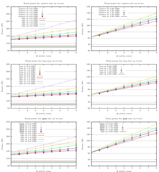
(6) 6. José I. Aliaga et al. Platform. P-state, Pi. PiY. αi. βburn,i. βbusy,i. βgemm,i. PiU. wt amd. P0 P1 P2 P3 P4. 84.83 77.85 73.83 71.86 72.46. 140.94 137.47 131.35 127.87 124.89. 14.70 7.71 5.48 4.12 3.10. 13.50 6.10 4.58 3.33 2.28. 13.82 10.01 7.40 5.46 4.27. 56.11 59.62 57.52 56.01 52.43. wt int. P0 P1 P2 P3. 33.43. 64.44 63.38 64.10 64.72. 9.48 8.19 7.33 6.34. 7.10 6.16 5.43 4.64. 11.12 9.84 9.03 7.81. 31.01 29.95 30.67 31.29. Table 2 Parameters for the simple power model for the cpuburn, busy and gemm benchmarks (kernels) on wt amd and C (c) = P C1 · c = β wt int. Note that PiU = αi − P Y and Pk,i k,i · c, with i, k and c denoting, respectively, the kernel type, k,i. P-state and number of cores.. levels, floating-point units, branch logic, etc.). While our power models refer to the power dissipated at a given instant of time t, in most experiments next, we will report instead the average power for the application, as this allows us to compile the information for the complete execution in a single figure. Furthermore, this easily connects the results with the total energy consumption. Given a platform with all cores in state Pi , for simplicity we will assume that PiY and PiU (i.e., the system and uncore powers in state Pi ) remain constant during the execution of the application. In practice, starting from an idle (cold) platform, these two factors grow with the system temperature till their addition reaches a plateau [12]. To avoid this effect, we assume that there is a continuous workload to run in the platform and, in order to mimic this situation, all our tests will be performed on a “hot” system, with this state reached by initially warming the cores with an execution of the same kernel or application for a given period of time. Also, we will assume that PiU is independent of the application that runs in the platform. In practice, this is not the case, but our results will show that the errors introduced by this simplification are small, and can be easily accommodated into the model. To obtain practical values for the power model, we proceed as follows. For simplicity, let us assume that all c active cores of the platform run the same type of task (kernel) k, in the same state Pi , during all the execution time. In this scenario, we can easily consider that the total power at instant t equals the average power. For PiY , we thus simply set all the cores of the platform to each P-state using cpufreq, and then measure the power with the platform idle. for 30 seconds and average the results: between 71.86 and 84.83 W, depending on the state Pi , for wt amd; and 33.43 W for all P-states in wt int; see column PiY in Table 2. The estimation of PiU and PiC is more elaborated, as it is difficult to separate these two components, and the second depends also on the application that is being run. In order to achieve this, let us start by refining (1), to capture the total power for the execution of c copies of task k, with the active cores in state Pi : T C C1 Pk,i (c) = PiY +PiU +Pk,i (c) ≈ PiY +PiU +Pk,i ·c, (2) C1 where Pk,i denotes the power dissipated by a single core in state Pi running task k. To estimate the missing parameters in (2), PiU C1 and Pk,i , we will leverage three compute-intensive kernels: the cpuburn microbenchmark3 , a simple busywait test consisting of a “while (1) ;” loop, and the general dense matrix-matrix product (gemm) routine implemented as part of Intel MKL operating with double-precision data. Specifically, we executed these tests for 60 seconds and averaged the power draw, for an increasing number of cores c (all in the same P-state) of the machines (8 cores of both wt amd and wt int), while the remaining cores remain in an inactive C-state. Applying linear regression to the data obtained from this experimental evaluation, we obtained linear models for the total power of the form T Pk,i (c) = αk,i + βk,i · c,. (3). 3 http://manpages.ubuntu.com/manpages/precise/man1/ cpuburn.1.html..

(7) Title Suppressed Due to Excessive Length. 7. Total power for cpuburn test on wt amd. Total power for cpuburn test on wt int 160. 350. Power (W). 250. at at at at at at at at at at. 2.0 1.5 1.2 1.0 0.8 2.0 1.5 1.2 1.0 0.8. GHz GHz GHz GHz GHz GHz GHz GHz GHz GHz. 140. cpuburn cpuburn cpuburn cpuburn idle. at at at at at. 1. 2. 2.00 1.87 1.73 1.60 2.00. GHz GHz GHz GHz GHz. 120 Power (W). 300. cpuburn cpuburn cpuburn cpuburn cpuburn idle idle idle idle idle. 200. 100. 80. 150 60 100. 40. 20. 50 1. 2. 3. 4. 5. 6. 7. 8. 3. # active cores Total power for busy test on wt amd. 6. 7. 8. 7. 8. 7. 8. 160 busy busy busy busy busy idle idle idle idle idle. at at at at at at at at at at. 2.0 1.5 1.2 1.0 0.8 2.0 1.5 1.2 1.0 0.8. GHz GHz GHz GHz GHz GHz GHz GHz GHz GHz. 140. busy busy busy busy idle. at at at at at. 2.00 1.87 1.73 1.60 2.00. GHz GHz GHz GHz GHz. 120 Power (W). Power (W). 250. 5. Total power for busy test on wt int. 350. 300. 4. # active cores. 200. 100. 80. 150 60 100. 40. 20. 50 1. 2. 3. 4. 5. 6. 7. 8. 1. 2. 3. # active cores Total power for dgemm test on wt amd dgemm dgemm dgemm dgemm dgemm idle idle idle idle idle. at at at at at at at at at at. 2.0 1.5 1.2 1.0 0.8 2.0 1.5 1.2 1.0 0.8. 6. Total power for dgemm test on wt int. GHz GHz GHz GHz GHz GHz GHz GHz GHz GHz. 140. dgemm dgemm dgemm dgemm idle. at at at at at. 2.00 1.87 1.73 1.60 2.00. GHz GHz GHz GHz GHz. 120 Power (W). Power (W). 250. 5. 160. 350. 300. 4. # active cores. 200. 100. 80. 150 60 100. 40. 20. 50 1. 2. 3. 4. 5. 6. 7. 8. # active cores. 1. 2. 3. 4. 5. 6. # active cores. Fig. 2 Power dissipated as a function of the number of active cores for kernels cpuburn, busy and gemm (top, middle and bottom, respectively) on wt amd (left) and wt int (right).. with the values for αk,i and βk,i in the corresponding columns of Table 2, and the relation between the models and the experimental data graphically captured in Figure 2. These regression models show quite a perfect fit with the experimental data, offering the same (rough) value αk,i for all three kernel types (the largest variation between the three was 2.11 % and the aver-. age difference 0.61 %.) Therefore, in the following we use αi − PiY as an estimation for PiU (see Table 2), the uncore power dissipated by a socket in state Pi (which agrees with our assumption that the uncore power is independent of the kernel type); and we set C C1 Pk,i (c) = βk,i · c so that Pk,i = βk,i ..

(8) 8. José I. Aliaga et al.. Thread Thread Thread Thread Thread Thread Thread Thread. 1 2 3 4 5 6 7 8 0 µs. 54.867.754 µs. Activity. Polling. Watts 193 67. Thread Thread Thread Thread Thread Thread Thread Thread. 0 µs. 54.867.754 µs. 1 2 3 4 5 6 7 8 0 µs. 54.867.754 µs. C0. C1. C6. Fig. 3 Traces of core activity, power and C-states (top, middle and bottom, respectively) during the computation of the ILU preconditioner using the performance-oriented, power-oblivious runtime, with all cores of wt int in state P0. Thread Thread Thread Thread Thread Thread Thread Thread. 1 2 3 4 5 6 7 8 54.342.740 µs. 64.234.465 µs. Activity. Polling. Watts 193 67. Thread Thread Thread Thread Thread Thread Thread Thread. 54.342.740 µs. 64.234.465 µs. 1 2 3 4 5 6 7 8 54.342.740 µs. 64.234.465 µs. C0. C1. C6. Fig. 4 Traces of core activity, power and C-states (top, middle and bottom, respectively) during (part of) the iterative solution stage using the performance-oriented, power-oblivious runtime, with all cores of wt int in state P0.. 5 Leveraging the C-States in ILUPACK We next investigate the exploitation of the C-states made by two implementations of the runtime underlying ILUPACK, and relate their costs to the previous power model. In the experiments in this section, we employ all the cores of the target platforms; and. we set the Linux governor to ondemand operating all the active cores in the same state P0 during all the execution (i.e., we do not allow voltage-frequency changes). In Section 2 we exposed that the task-parallel calculation of the preconditioner in ILUPACK is organized as a directed task graph, with the struc-.

(9) Title Suppressed Due to Excessive Length. ture of a binary tree and bottom-up dependencies, from the nodes (tasks) at each level to those in the level immediately above it. The subsequent iterative process basically requires the solution of (lower and upper) triangular linear systems per iteration, with tasks that are also organized as binary tasktrees, with bottom-up (lower triangular system) or top-down (upper triangular system) dependencies. In any case, when the tasks of these trees are dynamically mapped to a multicore platform by the runtime, the execution should result in periods of time during which certain cores are idle, depending on the number of tasks of the tree, their computational complexity, the number of cores of the system, etc. It is basically these idle periods that we could expect that the operating system leverages, by promoting the corresponding cores into a power-saving C-state (sleep mode). Figure 3 presents the execution trace, power consumption, and C-states observed during the computation of the ILUPACK preconditioner, using the original (power-oblivious) runtime, with all cores of wt int in state P0. Surprisingly, the results are quite different from what we had expected: Idle periods do not show a transition of the corresponding core to a power-saving C-state and the associated reduction of the power rate. Figure 4 reports an analogous behavior for the (preconditioned) iterative solution stage on wt int (and similar results were also obtained for both stages on wt amd). A closer inspection of the runtime that leverages the taskparallelism in ILUPACK reveals the reason for these surprising results. Concretely, in the original implementation of ILUPACK runtime, upon encountering no tasks ready to be executed, “idle” threads simply perform a “busy-wait” (polling) on a condition variable, till a new task is available. This strategy thus prevents the operating system from promoting the associated cores into a power-saving C-state because the threads are not actually idle (but doing useless work). This performance-oriented decision is far from uncommon, being adopted in runtimes like OmpSs (SMPSs) [28] or libflame+SuperMatrix [17] as well. Furthermore, the same performance-oriented but power-oblivious behavior appears, for example, when a synchronous GPU kernel is invoked with the default operation mode of CUDA [24] (the CPU remains in an active polling, waiting for the GPU to finish), or with the polling mode of certain MPI implementations (e.g., MVAPICH [23]).. 9. As an alternative to the previous power-hungry strategy, we developed a power-aware version of the runtime underlying ILUPACK, which applies an “idlewait” (blocking) whenever a thread does not encounter a task ready for execution and, thus, becomes inactive. (Note that setting the necessary conditions for the operating system to promote the cores into a power-saving C-state is as much as we can do, since we cannot explicitly enforce the transition from the application code.) As in the original version of the runtime, upon completing the execution of a task, a thread updates the corresponding dependencies identifying those tasks, if any, that have become ready for execution. However, in the power-aware runtime, the thread also ensures that the number of active (non-blocked threads) is, at least, equal to the number of ready tasks, releasing blocked threads if needed. The effect of idle-wait on the power trace and use of the C-states of wt int is illustrated in Figure 5, for the calculation of the preconditioner, and Figure 6, for the iterative solution stage. Compared with the performance-oriented (but power-hungry) implementation of the runtime (see Figures 3 and 4), the new runtime effectively allows inactive cores to enter a power-saving C-state, thus yielding the sought-after power reduction. The pending question, however, is whether the adoption of the power-aware runtime comes with a performance penalty which may blur the energy benefits, as in most cases the key factor is energy instead of power. Table 3 compares the execution time, average power, and energy consumption of the two runtimes, showing that fortunately this is not the case for the computation of the preconditioner and iterative solution, on any of the two target platforms when operating in state P0. Consider for example platform wt amd: For a minimal increase in the total execution time, from 286.28 s to 287.91 s, we observe reductions in the (average) power from 240.17 W to 227.16 W for the preconditioner; and from 269.27 W to 230.80 W for the solver. The outcome is a decrease of the total energy from 75,163.74 J to 67,758.84 J (−10.88 %). The power reductions attained by the power-aware implementation with respect to the power-oblivious case are given in percentage in the columns labeled as “Experimental” of Table 4 (averaged for 10 repeated executions). Combined with the negligible impact of the runtime on the execution time, these power figures also justify similar energy savings..

(10) 10. José I. Aliaga et al.. Thread Thread Thread Thread Thread Thread Thread Thread. 1 2 3 4 5 6 7 8 0 µs. 56.342.740 µs. Activity. Blocking. Watts 189 30. Thread Thread Thread Thread Thread Thread Thread Thread. 0 µs. 56.342.740 µs. 1 2 3 4 5 6 7 8 0 µs. 56.342.740 µs. C0. C1. C6. Fig. 5 Traces of core activity, power and C-states (top, middle and bottom, respectively) during the computation of the ILU preconditioner using the power-aware runtime, with all cores of wt int in state P0. Thread Thread Thread Thread Thread Thread Thread Thread. 1 2 3 4 5 6 7 8 56.342.740 µs. 65.876.075 µs. Activity. Blocking. Watts 189 30. Thread Thread Thread Thread Thread Thread Thread Thread. 56.342.740 µs. 65.876.075 µs. 1 2 3 4 5 6 7 8 56.342.740 µs. 65.876.075 µs. C0. C1. C6. Fig. 6 Traces of core activity, power and C-states (top, middle and bottom, respectively) during (part of) the iterative solution stage using the power-aware runtime, with all cores of wt int in state P0.. Let us now relate the power-energy reductions attained by the reimplementation of the runtime that leverages the CPU C-states to the power model of the previous section. For this purpose, we need to i) account the periods of “idle” time during the execution of ILUPACK, with both the original and energy-aware variants, as well as ii) assess the im-. pact of replacing a busy-wait (polling) for an idlewait (blocking). In order to tackle i), we follow a pragmatic approach, and simply execute the actual codes and measure the actual idle and computation times in our case, e.g., using the tracing framework Extrae+Paraver, while collecting power samples with the internal wattmeter and pmlib library..

(11) Title Suppressed Due to Excessive Length. 11. Platform. Runtime type. Time. Preconditioner Power Energy. wt amd. Oblivious Aware. 66.11 66.52. 240.17 227.16. 15,878.82 15,112.06. 220.17 221.39. 269.27 237.80. 59,284.92 52,646.41. 286.28 287.91. 75,163.74 67,758.84. wt int. Oblivious Aware. 54.01 54.47. 137.58 125.70. 7,431.67 6,847.47. 146.67 148.15. 162.34 150.17. 23,809.87 22,247.93. 200.68 202.62. 31,241.69 29,095.40. Time. Iterative solver Power Energy. Time. Total Energy. Table 3 Execution time, average power and energy of the power-oblivious and power-aware implementations of the. runtime (top and bottom, respectively) with all cores operating in state P0.. For ii), we use the data in Table 2 for P0Y , P0U ; C1 and estimate Pilu = βilu,0 using a procedure for ,0 ILUPACK analogous to that exposed for the three benchmark kernels combined with linear regression. Finally, we assume that a core promoted to a sleep state does not dissipate any core power. T T Consider Ppilu (c) and Pbilu (c) denote, respec,0 ,0 tively, the total power dissipated during the execution of ILUPACK, using the power-oblivious (polling pilu) and power-aware runtimes (blocking bilu), with c cores in state P0. Since now some cores may be inactive during a certain part of the execution, we need to adapt (2), which now becomes T C1 Ppilu (c) = fpilu,0 · (PiY + PiU + Pilu · c) ,0 ,0. + (1 − fpilu,0 ). (4). C1 · (PiY + PiU + Ppolling · c). ,0. The first term of the addition captures the cost of the cores performing useful work during the computation of ILUPACK (like (2)), and appears multiplied by fpilu,0 , which corresponds to the ratio of the total time that this computation occupies. Thus, the second part of the addition represents the remaining fraction of the total time, (1 − fpilu,0 ), and captures the power dissipation of the cores performing polling. C1 C1 In our evaluation, we set Ppolling = Pbusy , as the ,0 ,0 underlying procedures are similar. T On the other hand, for Pbilu (c), we have ,0 T C1 Pbilu (c) = fbilu,0 · (PiY + PiU + Pilu · c) ,0 ,0. + (1 − fpilu,0 ) · (PiY + PiU ),. (5). as we assumed that a core in blocking mode wastes C1 no power (i.e, Pblocking = 0). ,0 Table 4 compares the values of the theoretical raT T tios Pbilu (c)/Ppilu (c) with the experimental data ,0 ,0 (averaged for 10 different executions), showing a very. close matching between the two, below 2 %, wt int and slightly larger, about 4 % for wt amd. These results confirm the benefits of the power-aware runtime, but also the accuracy of the power model. For all other frequencies, as we will see next, the model always predicted the power-ratio with an error below 2 %.. 6 Impact of the P-states on ILUPACK In this section we evaluate the effect of the different P-states available for each processor on the performance-power-energy trade-off of ILUPACK. For that purpose, we set the Linux governor mode to userspace, and operate all the cores of the platforms in the same P-state. In the following, we always employ the power-aware version of the runtime. Therefore, we assume that, when idle, a core will remain in one of the deep power-saving C-states (C1 or higher), consuming a negligible amount of power. The general consensus is that, for a memorybound computation, some benefit may result from operating the system cores at low frequencies. The reason is that, although there exists a linear dependence between the core performance and the frequency, the effect on the execution time of a memorybound algorithm should be minor because the key for this type of computation is not core performance but memory bandwidth. On the other hand, for current multicore technology, a reduction of frequency is associated with a decrease of voltage (see Table 1) and, because of the relation between static power to V 2 and dynamic power to V 2 · f , in principle we can expect a significant reduction of the power draw. However, the balance between these two factors, time and power, on the energy efficiency is delicate, and other elements also play a role. Whether these variations of time and power yield a loss or a gain for ILU-.

(12) 12. José I. Aliaga et al.. Platform. Preconditioner Theoretical Experimental. Iterative solver Theoretical Experimental. wt amd. 89.58. 93.88. 91.47. 87.36. wt int. 90.11. 90.64. 93.65. 92.05. Table 4 Expected and observed (theoretical and experimental, respectively) power ratios, in %, between the power-. aware implementation of the runtime and the power-oblivious one, with all cores running in state P0.. Platform. P-state, Pi. Time. Preconditioner Power Energy. wt amd. P0 P1 P2 P3 P4. 66.52 81.56 97.16 113.25 137.62. 227.17 197.77 172.68 160.16 151.52. 15,112.06 16,131.31 16,778.25 18,138.44 20,852.36. 221.39 252.54 288.31 326.11 284.34. 237.80 207.98 187.14 176.10 167.36. 52,656.41 52,525.50 53,954.38 57,426.43 64,321.79. wt int. P0 P1 P2 P3. 54.47 57.31 60.65 65.29. 125.70 119.23 114.16 108.95. 6,847.47 6,833.73 6,924.03 7,114.07. 148.15 147.16 151.35 164.85. 150.17 145.37 140.75 132.35. 22,247.94 21,392.83 21,302.70 21,819.16. Time. Iterative solver Power Energy. Table 5 Execution time, power and energy of the power-aware implementation of the runtime, with all cores in state. Pi . Preconditioner ∆Power ∆Energy. Iterative solver ∆Power ∆Energy. Platform. Pi /P0. ∆fi. ∆BWi. −25.00 −40.00 −50.00 −60.00. −18.68 −32.45 −42.29 −53.78. 22.60 46.06 70.24 106.88. −12.94 −23.99 −29.50 −33.30. 6.74 11.02 20.02 37.98. 14.07 30.23 47.30 73.60. −12.54 −21.30 −25.94 −29.62. −0.22. wt amd. P1/P0 P2/P0 P3/P0 P4/P0 P1/P0 P2/P0 P3/P0. −6.50 −13.50 −20.00. −1.10 −0.86 −1.33. 5.21 11.35 19.86. −5.15 −9.18 −13.33. −0.20 1.12 3.89. −0.67. wt int. −3.20 −6.27 −11.86. −3.84 −4.25 −1.93. ∆Time. ∆Time. 2.16 11.27. 2.48 9.07 22.17. Table 6 Variations of frequency, bandwidth, execution time, power and energy ratios (%), of the power-aware imple-. mentation of the runtime, between state Pi and state P0.. PACK from the point of view of energy efficiency is thus the question to investigate in this section. Table 5 reports the impact of the P-states on the time, (average) power consumption and energy efficiency of the two stages of ILUPACK, calculation of the preconditioner and iterative solution, on both platforms. To help with the analysis of these results, Table 6 offers the variation ratios of bandwidth and the results that are experienced when moving from state P0 to state Pi , calculated as 100·(Mi −M0 )/M0 , where M0 and Mi denote, respectively, the values of the magnitudes (parameters or results) in states P0 and Pi .. The first aspect to notice is that the presumed independence between execution time and core frequency does not hold on wt amd. This should not be a surprise as our experiment in Table 1 already revealed that there is a strong connection between the core frequency and the memory bandwidth on this platform (see also column ∆BWi in Table 6). The combined decreases of frequency and memory bandwidth when moving from P0 to a higher P-state (between −25 % and −60 % for the former and from −18.68 to −53.78 % for the latter) explain the increases of execution time for both the preconditioning stage (22.60–106.88 %) and the iterative solver (12.54–73.60 %) in this platform. The behavior of.

(13) Title Suppressed Due to Excessive Length. 13. wt int is quite different, which is partially explained because now the reduction of frequency does not bring a decrease of memory bandwidth. Still, for the preconditioner, the reduction of frequency when moving from P0 to a higher P-state (−6.50 % for P1, −13.50 % for P2 and −20.00 % for P3), basically matches the increase of execution time for this stage (5.21, 11.35 and 19.86 %, respectively). We can take this as an indicator that the computation of the preconditioner (or, at least, parts of it) is not such a memory-bound computation as one could, in principle, presume. The results are different for the iterative solve. In this case, there is no significant difference in the execution time when running the stage in states P0 or P1, but the time increase when moving from P0 to P2/P3 is 2.16/11.27 %, which is still lower than what could be explained by the reduction of frequency alone. From the performance point of view, the major conclusion of this analysis is that the best solution is to always run ILUPACK with all the cores operating at the highest frequency (i.e., in state P0), though in some cases —in particular, the iterative solver executed in frequencies P0, P1 and P2—, the differences are small on wt int. Performance is crucial and, under some circumstances, energy efficiency is also vital. From that point of view, a reduction of power is beneficial only if it does not yield an increase of execution time that blurs the positive effects on energy consumption. For the particular case of ILUPACK, the results in Table 5 show that, on wt amd, the most energy efficient solution is to execute the preconditioner with all cores in state P0 but the iterative solver in state P1. For wt int, however, using states P1, P2 or P3 for the iterative solver results in small significant energy savings, from −1.93 to −4.25 %. Let us connect again the power variations attained with the different P-states and the models T for total power. For this purpose, we relate Pbilu (c) ,i T and Pbilu (c), using ,0 T C1 Pbilu (c) = fbilu,i · (PiY + PiU + Pilu · c) ,i ,i. + (1 − fbilu,i ) · (PiY + PiU ),. (6). and the experimental data. Table 7 reports the accuracy of our model to capture the experimental behavior due to the variations of the P-state on ILUPACK, with an error at most 3.08 % for wt amd and even smaller for wt int.. 7 Concluding Remarks We can list two main contributions for this work: i) the implementation of an energy-aware runtime for the complete preconditioner+iterative solve process in ILUPACK; and ii) the elaboration and experimental characterization of simple models for the (average) power that explain/justify the variations observed for the new energy-aware runtime and the effect of the different P-states for this particular application and two different multicore architectures. The introduction of the energy-aware runtime results from the experimental observation that, in an energy-oblivious execution of the original runtime for ILUPACK, idle threads with no useful task to execute simply poll till new work is available. As a result, these threads dissipate a significant amount of power in current processors, for no practical performance benefit for the particular case of ILUPACK. Our energy-aware implementation replaces this behavior with a more power-friendly implementation, that blocks idle threads till new work is available. This requires a careful reorganization of the underlying runtime, to avoid deadlocks and ensure a rapid response that does not impair performance. In our experiments, we observed savings in the energy usage between 7 and 13 %, at practically no cost from the performance point of view, which are clearly connected to the impact of the C-states by our power model. In summary, the approach adopted in this paper is based on the exploitation of idle periods during the concurrent execution of a task-parallel version of ILUPACK for multithreaded architectures. By replacing the busy-waits of the runtime in charge of execution with idle-waits, we favor the introduction of race-to-idle, which in turn allows the operating system to promote the hardware into a more energyefficient C-state. We believe that the same technique can be applied to other task-parallel scientific codes and, as part of ongoing work, we are currently embedding this approach into a general runtime like OmpSs, modified to embrace idle-wait, so that we can evaluate the performance-power-energy tradeoffs for other task-parallel applications. Busy-wait and idle-wait are analogous to wellknown concepts of operating systems like spinlock and mutex, respectively. The reason that idle-wait is beneficial for ILUPACK is that the number of changes between busy and idle periods is moderate.

(14) 14. José I. Aliaga et al.. Platform. wt amd. wt int. Pi /P0 P1/P0 P2/P0 P3/P0 P4/P0 P1/P0 P2/P0 P3/P0. Preconditioner Theoretical Experimental 88.05 78.96 73.50 69.73 95.62 90.84 87.21. 85.48 76.38 70.78 66.65 95.54 90.80 86.94. Iterative solver Theoretical Experimental 84.17 76.56 71.60 68.77 96.47 91.25 85.96. 87.64 79.65 74.85 70.80 96.47 91.84 87.77. Table 7 Expected and observed (theoretical and experimental, respectively) power ratios (%), of the power-aware. implementation of the runtime, between state Pi and state P0.. and the duration of these periods is “long enough”. This depends on a number of factors including not only the number and duration of the periods but, e.g., also the costs in time and energy of blocking/releasing the threads, the costs in time and energy of the changes between different C-states, etc. In theory, there exists a linear relation between performance and frequency, which could be expected to be even sublinear (at least on the Intel processor) for a presumedly memory-bound computation like ILUPACK, and a quadratic/cubic relation between energy and voltage-frequency. However, the analysis of the time-power-energy trade-off when the cores operate in a certain P-states (voltage-frequency pair), with the energy-aware version of the runtime, reveals the high impact of idle and, to a minor degree, uncore power which clearly favor shorter execution time over lower power dissipation rates. This is also contrasted to and accurately captured by our power model. Acknowledgments The researchers from the Universidad Jaume I were supported by project CICYT TIN2011-23283 of the Ministerio de Ciencia e Innovación and FEDER and the FPU program of the Ministerio de Educación, Cultura y Deporte. A. F. Martı́n was partially funded by the UPC postdoctoral grants under the programme “BKC5-Atracció i Fidelització de talent al BKC”. References 1. The Green500 list. Available at http://www.green500. org. 2. ILUPack. Available at http://www.icm.tu-bs.de/ ~bolle/ilupack/.. 3. The Top500 list, 2010. Available at http://www. top500.org. 4. Susanne Albers. Energy-efficient algorithms. Commun. ACM, 53:86–96, May 2010. 5. José I. Aliaga, Matthias Bollhöfer, Alberto F. Martı́n, and Enrique S. Quintana-Ortı́. Exploiting thread-level parallelism in the iterative solution of sparse linear systems. Parallel Computing, 37(3):183–202, 2011. 6. José I. Aliaga, Matthias Bollhöfer, Alberto F. Martı́n, and Enrique S. Quintana-Ortı́. Parallelization of multilevel ILU preconditioners on distributed-memory multiprocessors. In State of the Art in Scientific and Parallel Computing – PARA 2010, number 7133 in Lecture Notes in Computer Science, pages 162–172. 2012. 7. José I. Aliaga, Manuel F. Dolz, Alberto F. Martı́n, Rafael Mayo, and Enrique S. Quintana-Ortı́. Leveraging task-parallelism in energy-efficient ilu preconditioners. In 2nd International Conference on ICT as Key Technology against Global Warming – ICT-GLOW, number 7453 in Lecture Notes in Computer Science, pages 55–63. 2012. 8. P. Alonso, R. M. Badia, J. Labarta, M. Barreda, M. F. Dolz, R. Mayo, E. S. Quintana-Ortı́, and Ruymán Reyes. Tools for power-energy modelling and analysis of parallel scientific applications. In 41st Int. Conf. on Parallel Processing – ICPP, pages 420–429, 2012. 9. P. Alonso, M. F. Dolz, R. Mayo, and E. S. QuintanaOrtı́. Energy-efficient execution of dense linear algebra algorithms on multi-core processors, Cluster Computing, 16(3): 497-509, 2013. 10. P. Alonso, M. F. Dolz, R. Mayo, and E. S. QuintanaOrtı́. Modeling power and energy of the task-parallel Cholesky factorization on multicore processors. Computer Science - Research and Development, 2012. Available online. 11. M. F. Dolz, J. C. Fernández, R. Mayo, and E. S. Quintana-Ortı́. EnergySaving Cluster Roll: Power Saving System for Clusters. Architecture of Computing Systems - ARCS 2010, number 5974 in Lecture Notes in Computer Science, pages 162–173, 2010. 12. AnandTech Forums. Power-consumption scaling with clockspeed and Vcc for the i7-2600K. http://forums. anandtech.com/showthread.php?t=2195927, 2011. 13. S. Barrachina, M. Barreda, S. Catalán, M. F. Dolz, G. Fabregat, R. Mayo, and E. S. Quintana-Ortı́. An integrated framework for power-performance analysis.

(15) Title Suppressed Due to Excessive Length of parallel scientific workloads. In 3rd Int. Conf. on Smart Grids, Green Communications and IT Energyaware Technologies, 2013. 14. M. Duranton and et al. The HiPEAC vision for ad-. vanced computing in horizon 2020, 2013. 15. M. El Mehdi Diouri, M. F. Dolz, O. Glück, L. Lefèvre, P. Alonso, S. Catalán, R. Mayo, and E. S. QuintanaOrtı́. Solving some mysteries in power monitoring of servers: take care of your wattmeters! In Proc. Energy Efficiency in Large Scale Distributed Systems conference – EE-LSDS 2013, 2013. To appear.. 16. Wu-chun Feng, Xizhou Feng, and Rong Ge. Green supercomputing comes of age. IT Professional, 10(1):17 –23, jan.-feb. 2008. 17. FLAME project home page. http://www.cs.utexas. edu/users/flame/. 18. S. Gunther, A. Deval, and T. Burton. Energy-efficient computing: Power-management system on the Intel Nehalem family of processors. Intel Technology Journal, 15(1), 211. 19. D. L. Hill, T. Huff, S. Kulick, and R. Safranek. The Uncore: A modular approach to feeding the highperformance cores. Intel Technology Journal, 14(3), 2010. 20. HP Corp., Intel Corp., Microsoft Corp., Phoenix Tech. Ltd., and Toshiba Corp. Advanced configuration and power interface specification, revision 5.0, 2011. 21. J. Dongarra et al. The international ExaScale software project roadmap. Int. J. of High Performance Computing & Applications, 25(1):3–60. 22. J. Kolodziej, S. U. Khan, L. Wang, A. Byrski, N. MinAllah, S. A. Madani, Hierarchical genetic-based grid scheduling with energy optimization, Cluster Computing, 16(3): 591-609, 2013. 23. MVAPICH: MPI over InfiniBand, 10GigE/iWARP and RoCE. http://mvapich.cse.ohio-state.edu/. 24. NVIDIA Corporation. CUDA toolkit 4.0 readiness for CUDA applications, 4.0 edition, March 2011. 25. Paraver: the flexible analysis tool. http://www.cepba. upc.es/paraver. 26. E. Pinheiro, R. Bianchini, E. V. Carrera, T. Heath. Dynamic cluster reconguration for power and performance. In: Proc. of Workshop on Compilers and Operating Systems for Low Power, pp. 7593, 2003. 27. R. Schöne, D. Hackenberg, and D. Molka. Memory performance at reduced CPU clock speeds: an analysis of current x86 64 processors. In 2012 USENIX conference on Power-Aware Computing and Systems, 2012. 28. SMP superscalar project home page. http://www.bsc. es/plantillaG.php?cat_id=385. 29. The STREAM benchmark: Computer memory bandwidth. http://www.streambench.org/. 30. G. L. Valentini, W. Lassonde, S. U. Khan, U. Samee, N. Min-Allah, S.. Madani, J. Li, L. Zhang, L. Wang, N. Ghani, J. Kolodziej, H. Li, A. Y. Zomaya, C. Xu, P. Balaji and A. Vishnu, F. Pinel, J. E. Pecero, D. Kliazovich, and P. Bouvry, An overview of energy efficiency techniques in cluster computing systems. Cluster Computing, 16(1):3–15, 2013. 31. L. Wang, S. U. Khan, D. Chen, J. Kolodziej, R. Ranjan, C. Xu and A. Y. Zomaya. Energy-aware parallel task scheduling in a cluster. Future Generation Comp. Syst., 29(7):1661–1670, 2013.. 15.

(16)