Optimisation of a parametric cad geometry by means of a genetic algorithm

Texto completo

(1)TECNOLÓGICO DE M O N T E R R E Y ® INSTITUTO TECNOLÓGICO Y DE ESTUDIOS S U P E R I O R E S DE M O N T E R R E Y , MONTERREY CAMPUS. ENGINEERING DIVISION ENGINEERING G R A D U A T E S P R O G R A M M E. Thesis on Optimisation of a parametric CAD geometry by means of a genetic algorithm in partial fulfilment towards receiving the degree on Master in Sciences with specialization in Manufacturing Systems.. Presented by Edgar Francisco Ríos Soltero. Monterrey, N.L., México. August, 2010.

(2) W e the thesis committee members, recommend that the present work by Edgar Francisco ;. Ríos Soltero should be accepted as a partial requirement towards obtaining the academic degree of Master in Manufacturing Systems.. Dr. Arturo Galván Rodríguez. Dr. Hugo Ramón Elizalde Siller. (synodal). (synodal). (advisor). II.

(3) "Si vas a haceralgo,. hazlo bien". (If you are going to do something, do it right). Esperanza Ochoa. III.

(4) Table of contents Acknowledgements Abstract Abreviations Nomenclature Flowchart symbols 1 Introduction 1.1 Background 1.1.1 About the case study 1.1.2 Relationship between product design and computer intelligence 1.2 Problem definition 1.3 Hypothesis 1.4 Objectives 1.5 Scope and contributions 2 Theoretical framework 2.1 Genetic algorithms 2.2 The stress-strain diagram and the Von Mises' stress 2.3 A glance at finite element method 2.4 Parameters and features creation in computer-aided design 2.5 Materials and production processes 3 Proposed solution 3.1 Detailing a design concept 3.1.1 Set up of geometrical parameters 3.1.2 Design optimisation 3.1.3 Further improvement 4 Case study 4.1 Selection of the case study 4.2 Detailing a design concept 4.2.1 Set up of geometrical parameters 4.2.2 Design optimisation 4.2.3 Further improvement 4.3 Results 5 Conclusions and further work Appendix A - M A T L A B and CATIA interface library A.1 Comments about the interface Appendix B - Drawings of the mechanism Appendix C- Dynamic loading of the mechanism References. i iv v v vi 1 1 1 3 10 10 10 11 12 12 15 18 19 22 24 24 24 26 29 30 30 31 31 36 44 45 47 49 76 79 80 8. IV.

(5) List of figures Figure 1.1: Traditional damper 1 Figure 1.2: Diverse rotative applications using traditional dampers-(a) self-closing door[6], (b) landing gear[7], (c) deluxe cars[8], (d) bicycle seat[9], (e) training equipment[10] (f) specialised seats[11] and heavy machinery[12] 2 Figure 1.3: Different types of rotative dampers—(a) depends on rectilinear piston[4], (b) allows fullcycle[5], (c) depends on advanced materials[13] and (d) shows different designs based on the same mechanism[14] Figure 1.4: Process of F E M optimisation considering shape and manufacturability—taken from[25]....4 Figure 2.1: Genetic algorithms' analogy 13 Figure 2.2: The process of creating populations in G A 14 Figure 2.3: Qualitative stress-strain curves of representative materials (not at scale) 16 Figure 2.4: (a) States of Stress on an Element, (b) positive shear stress and (c) Negative shear stress (taken from [71]) 18 Figure 2.5: Equivalents to static mechanical problems—a cable under tension, a bar with a transverse load, a non-homogeneous bar with non-uniform transverse load, and a standing squared body (from top to bottom) 18 Figure 2.6: Multiple C A D operations—extrusion, revolution, protrusion, revolving protrusion, profile line-following, interpolating between multiple sections and filleting (from left to right) 21 Figure 3.1: Detailed design requires digitising a concept, establishing its parameters and optimising them 24 Figure 3.2: Definition of a circle—fixed definition (left) and parametric definition with a limit (right) 25 Figure 3.3: Optimisation cycle (GAà C A D àFEAàVMS) 27 Figure 3.4: Genetic algorithm used in this work 28 Figure 4.1:Disassembly of the damper mechanism for the case study (right) and assembly of the mechanism without the container. 30 Figure 4.2:Internal components of the mechanism in different positions 31 Figure 4.3: Definition of parameters (see Table 4.1) 32 Figure 4.4: Anchors in the axle and their counterparts in the piston 35 Figure 4.5: Flowchart showing the basic functions of the interface 37 Figure 4.6: Translating parameters' definition into mathematical expressions 38 Figure 4.7:Flowchart showing how to translate parameters' names and values into variables and mathematical expressions 39 Figure 4.8: Two perspectives of the finite element model set-up to be optimised (without the lid) 40 Figure 4.9: Flowchart showing the objective function of the A 43 Figure 4.10: Optimisation outcome—best evaluated phenotype 44 Figure 4.11: Further improvement of the geometry—the new anchor of the axle, its corresponding hole in the piston, the new orifices and minor radius of the valve, and the corresponding hole for the valve in the lid (from left to right) 45 Figure 4.12: Evolution of improvement (Von Mises' stress; left) and final geometry (right) 46 V.

(6) Figure 4.13: Mock-up Figure A.1:Geometry not prone to automatic meshing Figure A.2:Unsolvable analysis due to inability to apply boundary conditions Figure A.3:Unsolvable analysis due to topology change Figure C.1: Experimental arrangement to measure torque vs. angular speed Figure C.2: Plots of the same loading conditions of the mechanism with different valve positions— completely opened (top) and 75% closed (down). 46 76 77 77 80 81. VI.

(7) List of tables Table 1.1: Back-trace of computer intelligence for product design Table 2.1: Compatibility between processes and materials (augmented from [75]) Table 4.1: Definition of geometrical parameters' limits Table 4.2: Definition of geometrical parameters' limits Table A.1: Genotypes of the best evaluations for each generation Table A.2: Genes' equivalents for geometrical parameters Table B.1: Some important translations for the drawings. 9 22 33 36 75 75 79. VII.

(8) ACKNOWLEDGEMENTS I really don't like this word: acknowledgements. Rather, I would like to thank people, but I won't change the name of this section for the sake of formality. Another preamble: I will try not to mention any names to keep gals' and gents' privacy. I hope not to hurt anyone's feelings, so I will do this in a chronological way. Having said that, I would like to thank my family. I would not have wanted to do anything without their support. This includes my aunts, uncles, cousins, nephews, nieces and grandfather. I would like to especially thank a person who received me in Monterrey without any hesitations for as long as I needed it. I also thank a very good friend in that city who was always willing to give me a hand, whether it was picking me up or receiving me at his place. To all of my hometown's friends who I met in Monterrey. You were always a bastion to me. To the different sport teams and arts groups. To all of my other classmates who became good friends. These are only some of them; I can't remember all names, but I can surely remember our time together and what you did for me: L.D.G., E.S., G.B.M., O.L.M.C., D.M., R.S.C., R.C., J.F.H., B.C., E.M., A.M.B., C., H.J.F., O.C., H.R.E.S., D.E.C. and A.R. To the great teachers I had (disregard the lousy ones, please). About them, I remark A.V., M.A., J.A.G.L., P.P., J.I., J.L.L.S., G . E . Q . E . , A.G.R., J.L.G.V., O . R . V . , V N.J.H.T. and R.J.G. for being role models. To the people I met in the dinning. To my co-workers (not all of them, only the ones I really trust; if you are unsure, you should probably not ask). I note Claudia's immense help. To a good friend from my hometown who opened his house (or should I say couch?) when I most needed it. To all of my good friends in Purdue, even the little children. To a small paradise called Ithaca and all of its angels. To the exuberant tenderness of people around Kamitomioka road and all of the seibutsu support. To all of the Guards, Gardeners, Messengers, Executives, Doctors, Masters, Secretaries, Couch drivers i.

(9) and Cleaning-workers with whom I shared my days and nights. Especial thanks to all of those who bought cookies. I would like to greatly thank Marcelo (you never expected to see your name here, did you?. A tribute to you). Andrik, you are also a big part of this. Thank you a lot for what you did for me. I thank and acknowledge the support I received from Dr. Rafael Rangel Sostmann, Dr. Enrique Vogel and Maria del Rocío Diaz Vielba. You gave me hope when I felt lost. I will make my best to praise your effort through my work. At the same time, I thank Tec de Monterrey, Monterrey Campus and all of the good people who work to make it the best Mexican university. I am really grateful for having met such an outstanding group of people. Thanks to the Mexican Government and C O N A C y T for having supported me. ¡Tierra y libertad! Mr. Gonzalez provided insightful information regarding the performance of rotative mechanisms within prostheses; Dr. Goldfarb shared his perspectives on the. initial. development of the mechanism; Dr. Rivera and Dr. Garcia aided to establish the project's feasibility; Mr. Saldaña was always available to be consulted on D F M topics; Mr. Medina provided labour and knowledge for a preliminary mock-up of the device; Mr. Escarpita provided the idea of how to perform the viscosity coefficient tests of the mechanism; Mr. Vargas' commentaries on the feasibility of manufacture were very useful, and Mr. Yamin also advised on manufacturability. For this, I am compelled to acknowledge your efforts. Thanks to BASF© and Maincol, S.A. for their support. As a matter of copyright, I thank DragonArt. (http://dragonartz.wordpress.com). for. providing the original DNA helix used in figure 2.1. Besides, the support from the P L M lounge in CIDyT (Tec de Monterrey) regarding the use of the software was essential for this work. I ii.

(10) also thank all of the open-source community, you are great people. Any and all trademarks presented here are property of their respective owners, and the author takes no responsibility over them (this is an academic document). I would like to finish saying that it is evident that this report may have my name, but is clear that it is not my work alone. Thank you all.. iii.

(11) ABSTRACT This thesis has the aim of optimising a three-dimensional geometry whose dimensions have been previously defined by parameters. Such a definition allows the geometry to change its shape by altering the value of a parameter without the need of directly modifying a geometrical feature (extrusion, protrusion, etc.) itself. In this way, a single value may affect more than one characteristic of the design. Then, the task is to find the best combination of parameters which improve the performance of a design. In here, the optimisation is performed by the computer by means of a genetic algorithm to change the values of such parameters. There is extensive work in the subject of optimising the performance of products by means of genetic algorithms (GA). In this regard, much work has been done by using equations which model their behaviour. The widespread use of computerised technology (for design and analysis) eventually allowed researchers to combine G A with computer-aided design (CAD) and engineering (CAE). This resulted in two major branches of GA-based optimisation of geometries: the agglomeration of finite elements and the combination of geometrical features. In here, a G A is used to iteratively modify (in CAD) and evaluate (in finite-element analysis) a parametric geometry. This geometry corresponds to a mechanism recently developed by the author. The device has both dynamic and static characteristics, however, the evaluations (analyses) performed on the design are purely static An interface between a numerical analysis software (MATLAB1) and a C A D - C A E suite (CATIA1) is developed. The G A is run within the numerical analysis software and is interfaced to the C A D - C A E suite by means of its application programming interface (API). The results show the feasibility of improving a three-dimensional, feature-based and parametric C A D by means of the variations created by a G A . iv.

(12) ABREVIATIONS CI: computer intelligence G A : genetic algorithms NN: neural networks A C O : ant-colony optimisation P S O : particle swarm optimisation FL: fuzzy logic S A : simulated annealing 3D: three-dimensional 2D: two-dimensional C A D : computer-aided design C A M : computer-aided manufacturing C A E : computer-aided engineering C N C : computerised numerical control U N C : Unified National Coarse (thread) V M S : Von Mises' stress F E M : Finite Element Model (or Finite Element Modelling) F E A : Finite Element Analysis. NOMENCLATURE £: (epsilon, also lunate epsilon) strain v.

(13) ABREVIATIONS CI: computer intelligence G A : genetic algorithms NN: neural networks A C O : ant-colony optimisation P S O : particle swarm optimisation FL: fuzzy logic S A : simulated annealing 3D: three-dimensional 2D: two-dimensional C A D : computer-aided design C A M : computer-aided manufacturing C A E : computer-aided engineering C N C : computerised numerical control U N C : Unified National Coarse (thread) V M S : Von Mises' stress F E M : Finite Element Model (or Finite Element Modelling) F E A : Finite Element Analysis. NOMENCLATURE £: (epsilon, also lunate epsilon) strain v.

(14) : (delta) elongation length : (sigma) stress : modulus of elasticity : (epsilon) true plastic strain : strain-strengthening exponent (plastic stress); slope of a straight line (line equation); meters (length unit) : Pascals (pressure or stress unit) : Newtons (force unit) : inches (length unit) : yield stress : stress parallel to the. axis in the. : shear stress perpendicular to the. direction axis in the. direction. : radius of a circle : x-coordinate of a circle's centre : y-coordinate of a circle's centre : y-intercept of a straight line. FLOWCHART SYMBOLS Decision Transition file. Process Output file. Input or output Connector. vi.

(15) : (delta) elongation length : (sigma) stress : modulus of elasticity : (epsilon) true plastic strain : strain-strengthening exponent (plastic stress); slope of a straight line (line equation); meters (length unit) : Pascals (pressure or stress unit) : Newtons (force unit) : inches (length unit) : yield stress : stress parallel to the. axis in the. : shear stress perpendicular to the. direction axis in the. direction. : radius of a circle : x-coordinate of a circle's centre : y-coordinate of a circle's centre : y-intercept of a straight line. FLOWCHART SYMBOLS Decision Transition file. Process Output file. Input or output Connector. vi.

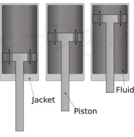
(16) Chapter 1 - Introduction. 1. INTRODUCTION 1.1. Background 1.1.1. ABOUT THE CASE STUDY. Traditionally, a damper is a mechanism which m o v e s in a rectilinear fashion[1]. Their main c o m p o n e n t s are: a jacket, a piston and a fluid. T h e inner geometry of the jacket is usually cylindrical, and contains a fluid that allows the piston to reduce its speed as it moves within the jacket. This is depicted in figure 1.1:. Figure 1.1: Traditional damper. Dampers are used as suspension systems or shock absorbers in many machines. Most people are familiar with the rectilinear type of d a m p e r s , because they have successfully been adapted to virtually any application. However, there are numerous examples in which the motion is not meant to be straight, thus, machines are modified to use this kind of d a m p e r s (see figure 1.2). The evident need for rotative d a m p e r s has led to their development. Their application has spread widely a m o n g commercial products (see figure 1.3). They are now used in niches which range from video recorders[2] to limb prostheses[3]. In each case, the design is adapted as required (see figure 1.3-d). S o m e of them are allowed to rotate full cycles[2],. 1.

(17) Chapter 1 - Introduction. s o m e depend on rectilinear pistons[4] and others require a d v a n c e d materials[5].. Figure 1.2: Diverse rotative applications using traditional dampers-(a) self-closing door[6], (b) landing gear[7], (c) deluxe cars[8], (d) bicycle seat[9], (e) training equipment[10] (f) specialised seats[ 11] and heavy machinery[ 12] This w o r k uses a damping mechanism which comprises a rotative piston, a viscous fluid and a rotating valve as its test subject for optimisation. It w a s recently developed by the author with the initial aim of being applied to trans-femoral prostheses. However, it is now being considered for a n y of the applications presented above (and more). A s it will be s h o w n later, the m e c h a n i s m has the ability to brake, but this d e p e n d s on its structural resistance. In this study, no dynamic nor d a m p i n g condition is used at all. It only contains the optimisation based on a static loading arrangement.. 2.

(18) Chapter 1 - Introduction. Figure 1.3: Different types of rotative dampers—(a) depends on rectilinear piston[4], (b) allows fullcycle[5], (c) depends on advanced materials[13] and (d) shows different designs based on the same mechanism[14] 1.1.2. RELATIONSHIP BETWEEN PRODUCT DESIGN AND COMPUTER INTELLIGENCE. It can be said that the w a y in which a product fulfils its requirements is through design parameters[15] a n d a series of parameters is what defines a product concept[16]. T h e definition of optimum values for these parameters is a complex task which c o n s u m e s valuable time in the product generation process[17]. Besides, their specification usually. requires. advanced knowledge or expertise in a given subject which m a y produce a relevant a n d unwanted bias[18]. Many authors have dealt with these issues through computer intelligence for structural and product design (see table 1.1). In the former, most of the w o r k has focused on finding the slimmest configuration b y removing material, a n d only some cases concern about the shape outcome. In the latter, the w o r k has centred on h o w to automate the creative process of concept generation through combining previously captured knowledge (databases of products or w a y s to perform functions). The table below (1.1) s h o w s the use of computer intelligence within the product design. 3.

(19) Chapter 1 - Introduction. niche. It can be seen that most of the research has focused on the use of genetic algorithms as a feasible tool to improve the required performance. T h e o n e with the broader scope from the artificial intelligence point of view is [19]. However, the w o r k from Lipson and Pollack[20] may also be remarked, because it m a n a g e s to take a concept a n d link it directly to a manufacturing process. T h e w o r k presented by [21] does not actually tackle the evaluation of designs, but could be helpful to determine inventive solutions. T h e w o r k from [22] c o m e s short in that it only modifies the positions of a 2D spline's points without ever considering topology, manufacturability or any other aspect of the design. Furthermore, spline-designing is rather difficult to c o m m u n i c a t e through drawings and to manufacture, all of which could lead to. infeasible. designs.. Actually,. there. are. some. authors. who. explicitly. focus. on. manufacturability[23]. S u n , Frazer and Mingxi[24] are still working on h o w to incorporate this particular issue into their work. Despite depending on the designer to decide w h e n to finish the optimisation process, they provide a very user-friendly interface to start the iterations. Their w o r k is also valuable, because they address multiple-parts products.. Figure 1.4: Process of FEM optimisation considering shape and manufacturability—taken from[25] There are m a n y works like the o n e presented by [25] in the sense that it addresses static structures. Nonetheless, this particular w o r k is worth mentioning, because it brings a leap in manufacturability (see figure 1.4). This type of w o r k (structure optimisation) keeps a relationship to [26], because they almost always use F E M m e s h e s which cannot be easily re generated into geometrical features. T h e approach used in [26] could help in this reversing process.. 4.

(20) Chapter 1 - Introduction. Besides the already mentioned s c h e m e s , a commercial software called C A T I A ® offers the optimisation of a single parameter in a design by m e a n s of simulated annealing. This is d o n e in such a w a y that a geometry is varied in terms of a geometrical parameter and processed in a FEA which works as the evaluating function. An important remark is m a d e before continuing: the assumption that computers have the ability to produce technological innovative solutions must be taken with caution[27]. "Design is an iterative process by nature: new information is generated with each step, and it is necessary to evaluate the results in terms of the preceding step"[15]. Even w h e n this could be the reason for the success of genetic algorithms in design applications, it is unlikely that they alone could achieve such a task. However, s o m e cases show that new concepts could be obtained using a combination of computer-intelligence techniques[28][27][19][29].. 5.

(21) 6.

(22) 1. The Helicopter Sizing and Performance Computer Program 7.

(23) 8.

(24) Table 1.1: Back-trace of computer intelligence for product design. 9.

(25) Chapter 1 - Introduction. 1.2. Problem definition. T h e geometrical optimisation of products is rather c o m m o n and may be t i m e - c o n s u m i n g . Also, h u m a n - b a s e d optimisation of geometrical parameters may generate an undesirable bias towards non-optimum solutions. Most of the w o r k in automatic optimisation of products' geometries has focused on improving a finite-element m e s h or combining previously captured concepts. In the first case, 3D C A D - b a s e d geometries have only been used to generate a first model from which the optimisation algorithm takes off. This eventually generates the need for re-capturing the geometry in a C A D environment. In the second case, the geometries are subjected to mixing their c o m p o n e n t s so that new and improved concepts may be achieved. However, the (engineering) performance of the new concept w o u l d actually be u n k n o w n . T h e closest approximation to using 3D C A D - b a s e d geometries can only change a single parameter. per optimisation. There. also exists a w o r k. on. multi-parameter. CAD-based. geometry optimisation, however, it can only improve the positions of a series of curve-defining points. This evidence s h o w s a need for a w a y to run multi-parameter optimisation on 3D geometries.. 1.3. Hypothesis. It is possible to use genetic algorithms to modify and evaluate a parametric 3D geometry captured in a computer-aided design software for optimisation purposes.. 1.4. Objectives. T h e main objective of this thesis is to develop a link between computer-aided design (CAD), finite element analysis (FEA) and genetic algorithms to define the near-optimum 10.

(26) Chapter 1 - Introduction. values of a series of parameters driving the geometry of a product.. 1.5. Scope and contributions. This w o r k takes a C A D geometry and optimises its s h a p e by changing the values of a series of its parameters. T h e s e must have been previously defined by the user and determine the geometry of the product's parts. T h e optimisation is performed via genetic algorithms (GA) by an interface developed and presented in this work. A sum of the m a x i m u m Von Mises' stress (VMS) value from all the parts is used as the GA's objective function. T h e restrictions on loading are the s a m e in all cases. S o m e boundary conditions are allowed to c h a n g e , but they are restored for the next analysis to take place. However, a penalty value is a d d e d w h e n this happens. A multi-part product is used as a case study. Only static analyses w e r e performed on each variation of the device. S o m e considerations have also been m a d e to account for manufacturability. T h e s e refer to the application of geometrical rules during the optimisation stage to fit standard tools. An intuitive graphical user interface is not provided. T h e user should be able to set parameters and use the F E M suite in C A T I A ® . M i n i m u m knowledge of M A T L A B ® is also required. T h e present w o r k will provide software which can interact with user-defined parameters of CATIA's (V5R18) products and parts, and that can run predefined static FEA on C A T I A .. 11.

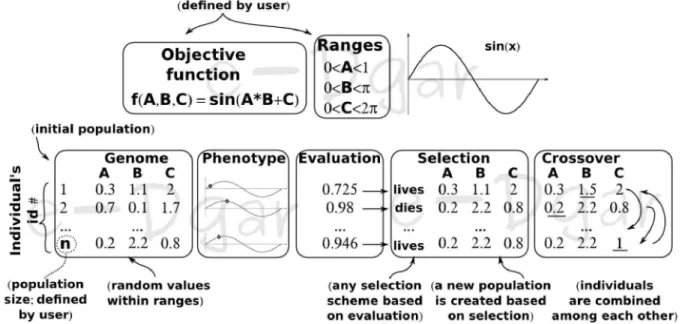
(27) Chapter 2 - Theoretical framework. 2. THEORETICAL FRAMEWORK 2.1. Genetic algorithms. Based on the definitions by Fulcher[27], it s e e m s reasonable to say that computer intelligence (CI) is a digital programmatic w a y of solving real-life problems by mimicking natural processes, may these be biological or not. For instance: s w a r m s , annealing, evolution, neural networks (NN), fuzzy logic (FL) or any other. This branch of informatics has been successfully applied to many subjects like medicine, economics and engineering (see [27], [19] and [29]). CI. is. rather. useful. "when. dealing. with. imprecise,. uncertain. and. incomplete. information"[19]. Nonetheless, it does have an inconvenience: "CI methods. require a. considerable a m o u n t of pre-processing (and, often,) parameter tunning"[27]. Therefore, the reader should keep in mind that their results d e p e n d greatly on the quality of the given inputs. Genetic. algorithms. (GA). are. the. computerized. analogy. of. evolution. applied. optimization problems[19] and the most c o m m o n kind of evolutionary computation techniques[27][68]. They w o r k with sets of w h a t. is called. individuals.. Each. to. (EC). individual. represents a tentative solution which is created from a combination of parameters called g e n e s . As it happens in nature, g e n e s comprise all of the information required to create an individual, and their combination results in the individual itself (the analogy of a phenotype). An evaluation is given to all individuals depending on a prepared testing function and their phenotype. This is used to select individuals, recombine t h e m with each other and obtain the fittest (or best) combination of parameters. The. following. picture. algorithms. At the top,. (2.1). shows. the analogy. between. real g e n e s. and. genetic. shows two different D N A strings being recombined into a new one.. In real individuals, the identification of D N A is customarily d o n e through serology which looks 12.

(28) Chapter 2 - Theoretical framework. as white a n d black stripes, represented by. In © , these stripes have been assigned with. binary a n d their corresponding decimal equivalents which m a y be interpreted by a computer. T h e phenotypes (the visual equivalent of genes), are s h o w n in. T h e r e , three spheres which. are different in size can be appreciated to depict that the biggest a n d the smallest balls are mixed into a n e w medium-sized o n e . A comparison between the values in © and the sizes of the radii in. s h o w s that a higher genetic value d o e s not guarantee a larger phenotype. T h e. phenotype will solely d e p e n d on the function which evaluates the values of the g e n e s . This is called an objective function, a n d is defined by the user.. Figure 2.1: Genetic algorithms' analogy T h e G A - b a s e d optimisation d e p e n d s on the evaluation of several individuals (see figure 2.2). More precisely, every optimisation step requires a set of individuals. Each n e w set is called a population, a n d its number of individuals is termed the population size. A s stated before, the individuals of a population are given an evaluation. This value is used for a selection process in which the worst phenotypes are disregarded (killed, deleted, etc.) and the best ones are duplicated. T h e genotypes of the fittest are then c o m b i n e d to create a new population. At the beginning, g e n e s are given a random value within user-provided ranges to create the first population. T h e creation and evaluation of each population is called a 13.

(29) Chapter 2 - Theoretical framework. generation. A n y other aspect of evolution m a y also be considered in G A . S o m e of these include migration, mutation, catastrophes, etc.. Figure 2.2: The process of creating populations in GA. It is a s s u m e d that the average evaluation of the population improves after several generations. This presumably occurs d u e to the combination of the characteristics of the best individuals a n d the removal of the worst. Actually, the average evaluation m a y as well stay the s a m e or be lower than the preceding population, but eventually increases with the passing generations. Any optimisation algorithm, including G A , is subjected to the restrains given by the user. T h e s e include the optimisation limits. T h o s e limits define a space (or hyper-space) of optimisation to which the algorithm is restraint. If the objective function is defined by a single parameter (or variable), the space b e c o m e s bi-dimensional, i.e. o n e axis for the variable a n d one for the function. Every. new parameter. corresponds. to a n e w dimension. of the. optimisation space. W h e n their number is very high, o n e m a y talk of a hyper-space. An advantageous characteristic of G A is that their solution is independent of the starting point in the optimisation space. Another very important feature of G A is that they only need a 14.

(30) Chapter 2 - Theoretical framework. w a y to evaluate the set of parameters for each individual[27][69][68]. This allows t h e m to be independent of derivatives or continuous mathematical functions.. 2.2. The stress-strain diagram and the Von Mises' stress. There exists a relationship between the stress of a body and its deformation. This relationship has been studied thoroughly for a vast a m o u n t of materials. It basically states that w h e n a body is subjected to a load, the size of the body changes. Depending on the load type, the dimensions may increase or decrease. For a given direction, this change is called stretch or elongation, and its ratio per unit length is called unit elongation or strain. This relationship is expressed as:. 5 where. {2.1}. is the total elongation of the bar within the length l and. is the strain[70].. T h e most c o m m o n expression to relate stress and strain is that of elasticity which is the property of a material to return to its original dimensions after a load has been applied to it. A linear relationship between the stress and strain w a s first stated by Robert Hooke, thus the n a m e Hooke´s Law. Many metals, ceramics and polymers have a regime of linear elasticity. T h e uni-axial expression of linear elasticity has the f o r m :. E€ so that. {2.2}. stands for the stress applied in the axial direction and. represents the modulus of. elasticity (also known as Young's modulus after T h o m a s Y o u n g ) , a constant of proportionality. Plasticity is another very c o m m o n concept relating materials' stress and strain. This p h e n o m e n o n occurs w h e n the material is not able to recover from deformation. Therefore, a material under plastic deformation will stay d e f o r m e d even after the load has been w i t h d r a w n . There are several. models. of plasticity,. but Datsko's. compact. expression. is. generally 15.

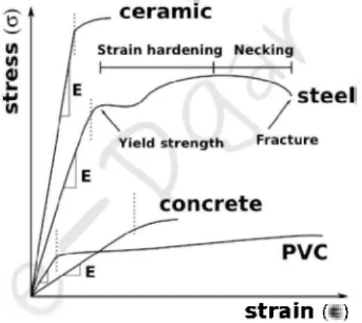
(31) Chapter 2 - Theoretical framework. accepted: £. in this case strain a n d. m. {2.3}. is a strength coefficient (or strain-strengthening coefficient),. is true plastic. is the strain-strengthening exponent[70].. T h e stress-strain behaviour of materials is usually represented in a graph called stressstrain diagram like the one shown in figure 2.3. In there, the linear elasticity zone of each material g o e s from the origin (no load) to the vertical d a s h e d lines. W h e n the m a x i m u m elasticity limit has been reached, the material yields a n d begins the plastic behaviour until it inevitable fractures. This yield strength is characteristic of each material a n d serves as a reliability parameter (aluminium: 4 0 0 M P a , steel: 4 6 0 M P a , d i a m o n d : 1 2 G P a , P V C : 7 0 M P a [approximate values; d e p e n d s on the composition]). It sets the point after which s o m e part of the deformation b e c o m e s permanent a n d non-reversible. For a given product, this m e a n s that its behaviour will probably no longer be the one for which it w a s designed or m a y not perform well.. strain (Є) Figure 2.3: Qualitative stress-strain curves of representative materials (not at scale). T h e discussion has only mentioned uni-axial stress. However, it is very unlikely that a material is subjected to pure uni-dimensional loads. In fact, the elastic properties of a material are three-dimensional. W h e n the loads on a material are equal in all three directions of a 16.

(32) Chapter 2 - Theoretical framework. Cartesian space, one refers to a hydrostatic condition. Experiments have s h o w n that under this circumstance, the yield strengths of materials are far higher than pure one-dimensional testing (like the ones in figure 2.3). This has led to hypotheses in which yield is related to the strain energy. Von Mises and Huber[71] proposed an approach in which the energy due to shape variations (commonly known as distortional energy) causes yielding. This can be expressed as:. σ´. 1. {2.4}. For the latter expression to m a k e any sense, the reader is advised to look at the following picture (figure 2.4) which presents the state of stress on a small material element. In there, the stress in the parallel direction to the to that s a m e axis is presented as. axis and which is applied to the face normal. . T h e s a m e definition may be applied to the y and z. axes. T h e s e stresses are known as the normal or axial c o m p o n e n t s of stress. An uni-axial loading condition comprises only one of these. On the other h a n d , the shear stresses are expressed as. . T h e s e generate angular deflections on the material. T h e nomenclature of. their sub-indices indicate the face on which they act j).. It is normally a s s u m e d that. and the direction of their application (. . If the loading condition of the element is k n o w n , the. value of equation {2.4} (the Von Mises' stress [VMS]) may be obtained.. 17.

(33) Chapter 2 - Theoretical framework. Figure 2.4: (a) States of Stress on an Element, (b) positive shear stress and (c) Negative shear stress (taken from [71]). 2.3. A glance at finite element method. T h e method of finite elements provides a w a y to solve equations, and is rather useful w h e n dealing with differential equations[72]. In solid mechanics, a finite element is a domain s e g m e n t e d by connecting elements, and each element is represented by a limited number of nodes. T h e s e are placed on the inter-element boundaries a n d possibly also within the element[73]. Problem. Free body diagram. FEM equivalent. Figure 2.5: Equivalents to static mechanical problems—a cable under tension, a bar with a transverse load, a non-homogeneous bar with non-uniform transverse load, and a standing squared body (from top to bottom) 18.

(34) Chapter 2 - Theoretical framework. Figure 2.5 s h o w s s o m e F E M equivalents to very basic static mechanical problems. Although much more complex problems may be solved by F E M , these examples serve to understand the transition from a real problem to a finite element m o d e l . It can be appreciated that to analyse a real-life problem, engineers translate it to free-body diagrams basically. indicate. the direction. and type. of. loads.. However,. in. FEM. the. which. problem. is. represented by nodes, elements and boundary conditions. For instance, the first element w o u l d be defined between node 1 (N1) and node 2 (N2). On each node, boundary conditions (BC) which correspond to each node w o u l d have to be applied. T h e s e have to comprise the loads and constraints of the problem, as well as the connectivity of elements. Besides segmentation, a F E M problem requires the selection of a mathematical model and a solution strategy. In fact, both the elements (number and type) and the method (model and solution strategy) used to describe their properties affect the accuracy of the results[73]. A more exhaustive model will probably output more complete results, but will also take longer. There are currently many front-end software applications to perform F E M so that the user does not have to worry about lengthy p r o g r a m m i n g . They can be classified as pre¬ processors, solvers and post-processors. T h e first class is used to set a n d , s o m e t i m e s , to s e g m e n t (usually called meshing) the problem. T h e second type uses this information and applies both a given model and a solution s c h e m e . Lastly, the third type interprets the results of the solver to calculate new values based on t h e m or display them graphically. There are also suites which integrate more than one of these processing classifications. More or less user input will be required for each task depending on the program.. 2.4. Parameters and features creation in computer-aided design. In product engineering, computer-aided design (CAD) refers to the use of computers to capture the geometry and geometry-related knowledge of designers into the computer. There. 19.

(35) Chapter 2 - Theoretical framework. are many C A D software available and they share many capabilities. For instance, it is now very c o m m o n that these applications allow both 2D and 3D drawings or representations of objects. There are both free, open-source and commercial C A D products available. T h e origin of C A D can be traced back to the 1970's. At the time, only manufacturable geometries. were. considered.. However,. a. breakthrough. on. how. the geometries. were. generated w a s achieved in the 1990's. That is, sketch-based graphical user interface (GUI) w a s introduced with the possibility of including constraints and d i m e n s i o n e d annotations. This allowed the creation of shapes from operations such as extrusion, revolution, protrusion or cut (see figure 2.6). This w a s d o n e in such a w a y that the sketches w e r e used to define those operations. This innovation also permitted to modify geometries by m e a n s of their constraints while assuring that the system can automatically create or modify related shapes accordingly. This requires parametric curves (circles, ellipses, etc.) to be incorporated and solved by C A D systems[74]. T h e use of sketches in C A D and constraint-based shapes introduces the need to fully define the curves. W h e n one of them is not fully defined, the C A D internally interpolates the rest of the data to fit the given dimensions. This case is known as a under-constrained sketch. A fully-constrained. (or well-constrained). sketch contains. all the information to set. the. drawings in space. However, the parameters need to be right or the curves cannot be created. Besides, there are s o m e cases in which the solver will not be able to plot a wellconstrained sketch. Many more a d v a n c e d capabilities have also been incorporated to C A D . T h e s e include the use of geometric constraints (parallelism, perpendicularity and so on) as well as equation systems, conditional or rules in which variables may be used as dimensional constraints[74].. 20.

(36) Chapter 2 - Theoretical framework. Figure 2.6: Multiple CAD operations—extrusion, revolution, protrusion, revolving protrusion, profile line-following, interpolating between multiple sections and filleting (from left to right). Depending on t h e C A D software, diverse geometrical features m a y be created (see figure 2.6). T h e s e include the already mentioned extrusion, revolution, protrusion a n d cut, but can be extended to filleting, sketch (or profile) line-following, section filling, interpolating a solid between t w o different curves, etc. T h e reader should remember that t h e successful creation of these features d e p e n d on both their correct definition a n d t h e internal graphicssolver within t h e C A D software. S o m e C A D also provide catalogues of standardised pieces, built-in programming environments, a d v a n c e d geometry creation (e.g. threads) a n d assembly capabilities.. 21.

(37) Chapter 2 - Theoretical framework. 2.5. Materials and production processes. Normal practice Less common Not applicable. Table 2.1: Compatibility between processes and materials (augmented from [75]). "(The) availability of materials a n d diversified processes in manufacturing has. allowed. complex product design"[76]. T h e criteria to choose between materials are (1) their physical and chemical properties, (2) the product's geometry[75], (3) cost a n d (4) production v o l u m e [ 7 7 ] . T h e first criterion (1) will determine the behaviour of a given geometry and its m e a n s to be produced (and/or assembled)[77]. In this w a y , the material a n d the w a y it is both produced a n d put together are collateral causes for the design's properties. There is very g o o d information regarding materials a n d processes provided by [75] a n d [78] which will not be presented here, but that can help the designer in the primary selection of materials a n d processes. Further data can be found in specialised handbooks a n d databases. Table 2.1 can 22.

(38) Chapter 2 - Theoretical framework. be of great help in the preliminary selection of manufacturing processes and materials. Boothroyd and Dewhurst[75] show a w a y to select the manufacturing processes and materials for a product. It is based on table 2.1 and on the s h a p e generation capabilities of each process.. 23.

(39) Chapter 3 - Proposed solution. 3. PROPOSED SOLUTION 3.1. Detailing a design concept. This section s h o w s the process to transform a rough representation of the design into the final concept. A s it is shown in figure 3 . 1 , this requires digitising the design in a t w o - or three-dimensional. drawing. software,. setting. specifications. (and/or. constraints). a n d the. application of an optimisation s c h e m e (genetic algorithms in this case). In most cases, the parameters. are (1) c h a n g e d. a n d (2) optimised. iteratively.. However,. these. are t w o. conceptually different processes, and need to be expressed separately to avoid confusion. Moreover, the w a y in which the optimisation is presented later in this d o c u m e n t requires a specific m e t h o d to define the geometrical parameters a n d their limits.. Figure 3.1: Detailed design requires digitising a concept, establishing its parameters and optimising them. 3.1.1. SET UP OF GEOMETRICAL PARAMETERS. Establishment of parameters is subjected to many factors. S o m e of these include the application of a certain design philosophy or method like product life-cycle, DfX or any company-specific. procedure. At the e n d , it is the geometry. that governs. the w h o l e. product[76]. It is a s s u m e d that a design concept is ready at this stage, so the actual matter is to determine. the parameters. which. it comprises.. These. a n d their. relationships. subordinated to the product's functionalities, inner interactions a n d feasible. will be. production. 24.

(40) Chapter 3 - Proposed solution. m e a n s . For instance, establishing parameters for sheet-metal artefacts requires very different types of constraints than those for mould-injected ones. Geometrical abstractions. (or topological). (notions,. limits will. ideas, sketches,. need. to be established. etc.) into the concrete. in order. (physical. to take. objects). T h e. relaxation of these limits permits wider variations of a single concept, but m a k e s the control of their relationships (and their optimisation) harder. T h e limits are established by m e a n s of simple mathematical inequalities with the aid of analytic geometry formulas. Firstly, the designer defines driving (independent) parameters as explicit values or ranges based on the product requirements. T h e n , based on t h e m , d e p e n d e n t parameters are expressed as equations or inequalities.. Figure 3.2: Definition of a circle—-fixed definition (left) and parametric definition with a limit (right) For instance (see figure 3.2), a w a y to produce a partial arc w o u l d be by defining a secant through a circle. T h e resulting shape w o u l d d e p e n d on exactly five parameters: the position of the circle's centre (a pair of coordinates) and its radius, and both the line's slope and its y-axis crossing-point (intercept). T h e s e parameters are expressed in the equations for the circle a n d the straight line: 2. r. 2. 2. (x-h ) + ( y-k ) y. = mx+ b. {31}. {32}. If the designer chooses to constraint the five parameters to single values, the design can be considered as finished. Conversely, if at least one of t h e m can be modified freely, there is 25.

(41) Chapter 3 - Proposed solution. an infinite number of possible geometrical combinations. W h e n limits are e s t a b l i s h e d instead, 2. there is a range of possible outcomes. For example (see figure 3.2), it could be possible to relate the radius of the circle to its distance to the x-axis. In this w a y , if the line is set to be the axis itself, t h e length of t h e resulting arc w o u l d be given by t h e mathematical function which relates t h e m . Moreover, setting limits for the distance (k <r<2k ; see figure 3.2) makes it easier to (1) know that the geometry will always look as an upright quasi-circle a n d (2) constraint it to never be less than a semi-circle. This is an example of how parameters define concepts. The process above m a y be simplified by C A D software's graphical user interface (GUI). In this w a y , a n intuitive interface m a y be used instead of actual mathematical expressions (or programming) to generate all kinds of geometries. S o m e companies even provide suites to undertake computer aided design, manufacture and/or engineering ( C A D / C A M / C A E ) in a single environment.. 3.1.2. DESIGN OPTIMISATION. W h e n parameters a r e set, the next step is to determine what is t h e best combination of values for a given concept. This c a n be done by means of computer intelligence, so a s to avoid the difficult task of refining the parameters: "Finalizing the specifications is difficult because of trade-offs—inverse relationships between two specifications that are inherent in the selected product concept. Trade-offs frequently occur between different technical performance metrics and almost always occur between technical performance metrics and cost The difficult part of refining the specifications is choosing how such trade-offs will be resolved."[17] Now, consider the optimisation possibilities as "a multidimensional surface in space a n d that the points on this surface represent different combinations of t h e design variables that can be reached. All points on the surface are various realizations of a single concept"[16]. A s. 2 The upper and lower values can also be considered driving parameters 26.

(42) Chapter 3 - Proposed solution. optimisation tools, the purpose of G A is to find the point with the best evaluation, in other w o r d s , the best concept. Since the G A only need a numerical evaluation for each combination of parameters, they can use the output of a FEA application (or other kind of software that can evaluate a C A D concept in any degree) as the objective function. In this case, the V M S result of a static analysis w a s used. In this w a y , the G A is responsible for modifying the values of the parameters which control the geometry of a design concept. T h e n , the F E A software is called to perform the static analysis of a given geometry as the objective function. At the end of the analysis, the value of the V M S is used as the evaluation given to the specific geometry variation. T h e n , the optimisation continues via the G A . This process is depicted in the following picture (figure 3.3).. Figure 3.3: Optimisation cycle (GA CAD. FEA. VMS).. T h e above process has t w o basic initial requirements. Firstly, the C A D model must be prone to geometrical parametrisation. In other w o r d s , the geometrical values of the model have to be linked to a variable, w h e r e these variables will b e c o m e the G A optimisation parameters. T h e link must be such that once the value of the variable is c h a n g e d , the geometry is modified accordingly. This implies that the C A D environment requires either internal programming or being able to receive a n d process the parameters' values from the outside. Secondly, the F E A software must be capable of receiving a C A D model a n d translate it into F E M . This includes a w a y to convert the geometry into a mesh a n d to apply the. 27.

(43) Chapter 3 - Proposed solution. appropriate restrictions and loads as boundary conditions in the right place. T h e software must also have internal programming capabilities or a w a y to output the result of the analysis. If these capabilities are not available by a single software, they must be guaranteed by any m e a n s possible. Fortunately, C A T I A ® can d o both.. Figure 3.4: Genetic algorithm used in this work. T h e genetic algorithm used here begins by creating random values within the range for each g e n e . T h e n , every individual is evaluated a n d undergoes tournament selection a m o n g its adjacent pair. That is, the worst evaluation is dismissed a n d replaced by the best o n e . T h e n , a permutation is performed to select which individuals in the population will crossover in random positions. W h e n this happens, new individuals with different g e n o m e s are created. 28.

(44) Chapter 3 - Proposed solution. T h e s e receive a phenotype and the cycle starts again (see figure 3.4). T h e surviving and unmodified individuals do not require the phenotype to be regenerated, because. their. previous evaluation is kept in the following population. The close relationship between the correct set-up of the geometrical parameters and their optimisation should now be clear.. 3.1.3. FURTHER IMPROVEMENT. S o m e times, an optimal solution is not possible (an approximated solution is termed near-optimal under these circumstances). In s o m e cases, the optimisation requires post¬ processing (e.g. due to simplifications in the model statement). It could also occur that new improvements or unforeseen attributes could arise during the optimisation stage. It should also be considered that the results could show important w e a k n e s s e s of the concept. A g o o d parametrisation makes this scenario less likely, but it could happen that the designer will need to redo the specification of parameters. Backtracking alternatives may be used to reinstall previous ideas as needed[79].. 29.

(45) Chapter 4 - Case study. 4. C A S E STUDY 4.1. Selection of the case study. A case study regarding a d a m p e r w a s c h o s e n . This d a m p e r is designed for rotative applications a n d claims to have the capability of intermediate breaking. This capability d e p e n d s on the structural resistance of its c o m p o n e n t s . S o m e parts of the m e c h a n i s m roll or are in direct contact with each other. Thus, the geometry greatly determines its performance. That is, if any of those c o m p o n e n t s fails, the product w o u l d cease to w o r k properly. Therefore, it s e e m s fundamental to find the optimum combination of parameters that enable the m e c h a n i s m to withstand static-loading conditions.. Figure 4.1:Disassembly of the damper mechanism for the case study (right) and assembly of the mechanism without the container. T h e device is internally flooded with a viscous fluid. Figure 4.1 and figure 4.2 show that the axle a n d the piston are joint and rotate as o n e . T h e container, the axle a n d the piston are a s s e m b l e d in such a w a y that the piston is internally mounted on the container. This creates a c h a m b e r into which the fluid is poured (represented as multiple dots in figure 4.2). T h e n , the lid closes this chamber. T h e fluid m a y be pushed through the orifices in the valve from o n e side to the other. However, it is not allowed to pass w h e n the valve is closed. Therefore, the piston a n d the axle are not allowed rotate under this circumstance. This is h o w the 30.

(46) Chapter 4 - Case study. m e c h a n i s m brakes, i.e. the set-up to be analysed.. Figure 4.2:Internal components of the mechanism in different positions. The m e c h a n i s m is fixed by the top planar face of the container, and the load (a torque) is applied on the orifices of the axle. The applied torque has the s a m e direction as the curved arrows in figure 4.2. The reader may notice from figure 4.1 that the piston is mounted on the axle by m e a n s of an anchor, and the valve is mounted on both the container and the lid. The lid is fixed to the container by setting screws (not shown). The m e c h a n i s m includes m a n y of the most c o m m o n geometrical features available in C A D software. Besides, it comprises the definition of advanced ones (e.g., threads). It also requires static analysis concerning contacting and rolling interactions. Its geometry is innerly related to its mechanical performance, and may be defined by a series of parameters. Therefore, it is suitable as a testing subject for this work.. 4.2. Detailing a design concept 4.2.1. SET UP OF GEOMETRICAL PARAMETERS. The first step in this process consists in identifying the governing parameters. The next figure (4.3) s h o w s the nomenclature used for the parameters and the geometry to which their values are related. T h e figure presents s o m e section views of the m e c h a n i s m which present all the dimensions that define the geometry of the device. In there, the longer distances w e r e taken as the driving parameters and the subsequent smaller ones w e r e defined as their. 31.

(47) Chapter 4 - Case study. fractional values. For instance, the value of AnchorMen hundred percent of AnchorMay.. may be between fifty and one. A table (4.1) is provided below to show the limits of each. parameter. S o m e of the limits are expressed in terms of other parameters and s o m e have been defined as numerical values.. Section view A-A Scale: 1 : 1. Figure 4.3: Definition of parameters (see table 4.1). Figure 4.3 s h o w s a dimensioned geometry w h o s e actual values have been omitted. T h e only purpose of these drawings is to facilitate the definition of the parameters' limits which will be optimised. Therefore, their exact values will b e c o m e relevant only after the optimisation process. S o m e of the dimensions are not s h o w n , because they are considered 32.

(48) Chapter 4 - Case study. as constants rather than parameters. However, they must be defined in the C A D software. T a k e the position of the five peripheral holes in the lid as an e x a m p l e : They have been designed so that they fall just in-between the two outer-most walls of the container. T h u s , they are not precisely defined by the user, but set by the geometry.. Table 4.1: Definition of geometrical parameters' limits. In spite of being driven by the longest parameters, it is r e c o m m e n d e d that the smallest are defined first. This enables the designer to set limits so that topology issues are less likely. For example, (see table 4.1 and figure 4.3) it is important to know which is the m i n i m u m value of AxleRollerX. (axle's distance between farthest parallel faces) w h e n defining. ContFront. (container's length between most distant parallel faces). Setting the value of the latter so that. 33.

(49) Chapter 4 - Case study. it is greater than the former avoids the creation of an axle which can't fit the container. T h e s a m e process should be used recursively for all the parameters. Table 4.1 also s h o w s several basic mathematical operations so that the reader can trace this process, but they actually represent single n u m b e r s . However, the definition of the parameters is still incomplete. T h e y require considerations on the tools and processes by which the parts will be p r o d u c e d . Firstly, plastics are not considered because (1) CATIA's FEM can only model linear (elastic) behaviour and (2) V M S w a s selected as the evaluating function of the geometries. This m e a n s that the results w o u l d only be valid for small stresses which is not expected in the real c a s e . T h e next viable selection is to c h o o s e metals, because they are not as brittle as ceramics and m u c h less expensive than carbon-based materials like carbon fibre. There are many options in this regard (iron, steel, titanium, a l u m i n i u m , etc.). In spite of a w i d e availability of manufacturing processes for metals, manual (not C N C ) machining w a s chosen as the main process for fabrication. This w a s d u e to availability, finishing requirements (rolling a n d sealing between parts) and cost for small v o l u m e s . Therefore, a new version of the limits is mandatory. Table 4.2 shows the new definition of the limits taking the manufacturing process into account. T h e reader may note a continuous transformation between milimeters and inches all along (25.4mm = 1in). This is d u e to the fact that Mexican machining shops are more likely to have imperial-sized tools. T h u s , w h e n a follows:. tool is required, a conversion is performed as. . For instance, the anchors which join the piston and axle are partly. defined by the parameters AnchorMay. and AnchorMen.. T h e first of these (see the section cut. D-D in figure 4.3 and figure 4.4) sets the total width of the anchors, while the second defines their internal width (after a c h a m f e r ) . However, this particular feature must be both externally and internally m a c h i n e d . That is, the anchors of the axle require a profiling, while their. 34.

(50) Chapter 4 - Case study. counterparts in the piston require pocketing operations (see figure 4.2). This. pocketing. requires a cutting tool with a m i n i m u m radius. In this case, the smallest tool diameter is a s s u m e d to be. . Therefore, the m i n i m u m width specification for both the axle a n d the. piston should be according to that diameter. This is established in the n e w definition of the m i n i m u m size for AnchorMen. in table 4 . 2 . Similar decisions w e r e m a d e for the rest of the. parameters.. Figure 4.4: Anchors in the axle and their counterparts in the piston.. 35.

(51) Chapter 4 - Case study. Table 4.2: Definition of geometrical parameters' limits. 4.2.2 DESIGN OPTIMISATION The w a y in which the geometrical parameters w e r e defined (see section 4.2.1) makes the optimisation easier by allowing a n y value between zero a n d o n e to set the values of driven parameters of the product. T h e s e values are set within a numerical analysis software ( M A T L A B ® ) by m e a n s of a genetic algorithm created by Dr. Manuel V a l e n z u e l a . The w a y in 3. which it w o r k s is by interpreting a minimum a n d a m a x i m u m a s the limits of a range for every defined variable (see section 3.1.2). 3 This code is not published due to copyright issues. The reader can consult Dr. Valenzuela at. or 36.

(52) Chapter 4 - Case study. Although the optimisation algorithm is run from M A T L A B ® , the objective. function. d e p e n d s on the result of a F E A which is run within C A T I A ® . Therefore, an interface between the t w o w a s fundamental. This interface w a s also used to apply the values generated by the G A to the parameters a n d update the phenotype (geometry) of the individuals. T h e next diagram (figure 4.5) s h o w s the basic functions of the interface.. Figure 4.5: Flowchart showing the basic functions of the interface. Firstly, the user must supply the n a m e s of C A D a n d F E M files. Next, the interface determines if such files exist, a n d asks for n e w n a m e s (or termination) to the user if that is not the case. W h e n the files are f o u n d , they are o p e n e d in a (non-visible) instance of C A T I A ® by m e a n s of its application programming interface (API). A variable is created so as to control the files from within M A T L A B ® . This allows access to the parameters defined in the C A D file. T h e user also has to provide the n a m e s of the parameters a n d their limits to the program in a separate file (considerations have been m a d e in the interface to facilitate its creation). T h e n , the interface converts these n a m e s a n d limits into a separate file which will later be used to calculate the values of the parameters within the specified range. Another set of variables (factors) are used to set the random values of the parameters. T h e G A is called once everything has been set (see figure 3.3). At the e n d , the results are presented in C A T I A ® a n d in a M A T L A B ® plot. There are many functions a n d subroutines involved in the process above. However, it is important to note s o m e of t h e m . For example, the program which runs the so mentioned process m a y be found in Appendix A under the n a m e e j e m p l o O p t i m . m . Another important matter is how to translate the n a m e s a n d the values of parameters into variables a n d mathematical expressions. A graphical representation has been prepared for the reader in 37.

(53) Chapter 4 - Case study. figure 4.6:. Figure 4.6: Translating parameters' definition into mathematical expressions. Put in w o r d s , the text file contains three columns separated by tabulators. T h e first contains the n a m e of the parameter which is translated into a variable that M A T L A B ® can interpret during the G A . T h e n , the contents after the second comparison symbol are copied into a mathematical expression, a n d then the data before the first comparison symbol is subtracted from it. T h e result is then multiplied by a factor which can g o from zero to o n e . Later, this will be taken as a g e n e by the G A . At the e n d , the data preceding the first comparison symbol is a d d e d to form the final expression. T h e s e functions are performed by archPars.m and a d q P a r a m . m (in Appendix A ) . T h e next diagram (figure 4.7) represents their code to help in the understanding of h o w this is d o n e . Although it is not s h o w n in the d i a g r a m , the output file m a y be written or modified manually.. 38.

(54) Chapter 4 - Case study. Figure 4.7:Flowchart showing how to translate parameters' names and values into variables and mathematical expressions. T h e reader may find that the last line of the flowchart in figure 4.7 starts with rounding up dimensions to a given factor. T h e reason for this is that using manual machining (turning a n d milling) as the manufacturing process allows the selection of parameters to be limited to t h e geometry of t h e tools. A quick examination of the geometry will show that the product only requires turning, thread tapping a n d milling. Therefore, to avoid infeasible dimensions in manufacturing, s o m e rules have been applied to the optimisation. T h e s e are: •. t h e m i n i m u m diameter to mill the holes in the valve w a s set to an eight of an inch,. •. the only two holes in the axle w e r e set to at least three sixtieths of an inch,. 39.

(55) Chapter 4 - Case study. •. the m i n i m u m diameter to mill the axle w a s set to three eights of an inch, a n d. •. any change in the parameters w a s set to 0.0005 of an inch. Since the optimisation uses a FEA, s o m e c o m m e n t s are needed regarding the F E M of. the product as well. First, o n e should remember (see section 2.2) that the linear behaviour d e p e n d s on the Young's modulus a n d that it is modelled as a slope parting from the origin. A m o n g ductile materials, this behaviour is quite similar. Therefore, aluminium w a s chosen for the F E M optimisation because it is rather c o m m o n a n d it has a much lower strength than steel (it could serve as a safety margin). T h e F E M used here performs t w o static stress analyses. T h e automatic. meshing. capability of the F E M software w a s used for both. T h e s u m of the t w o m a x i m u m V o n Mises' stresses w a s used as the evaluation of the individuals.. Figure 4.8: Two perspectives of the finite element model set-up to be optimised (without the lid). T h e first analysis uses a torque of 50N-m (represented as quasi-circles in Figure 4.8) on the internal holes' faces of the axle, a n d a clamp (zero degrees of freedom) on the planar face of the container. O n e of the frontal faces of the piston is held by a planar displacement constraint (i.e. it m a y slip on it, but cannot rotate or move in its normal direction). All the adjacent faces of the parts are allowed to slip on each other. A n hydrostatic pressure of 500 kPa is also applied on all the faces of the parts within the container. T h e lid (not s h o w n in 40.

(56) Chapter 4 - Case study. Figure 4.8) and the container are fixed to each other by (rigid) bolt connections, one on each of their respective five holes. T h e second analysis also uses the three last. boundary. conditions and a distributed force on the valve, perpendicular to the axle and the planar face of the container. All of the information provided so far makes it possible to introduce the objective function of the GA, i.e. the one that evaluates every individual. It is useful to keep in mind figure 3.3 and the process depicted in figure 3.4 for this. T h e function is represented in the flowchart of figure 4.9. It begins with a conditional using a counter, because experience s h o w e d that infinite loops which eventually used all of the available R A M of the computer w e r e occurring. This behaviour a p p e a r e d approximately once every ten individuals, i.e. w h e n trying to perform the optimisation of the tenth individual's geometry. Therefore, a restart w a s forced upon the C A D and F E M files. T h e s a m e problem s e e m e d to appear if a previous optimisation had taken a considerable amount of time. T h u s , a time-stamp w a s also consulted from. a. previously created text file (probably empty the first time) every time a new individual w a s about to be created. T h e optimisation did not s e e m to enter into the so mentioned loop again after this tuning. T h e objective function continues by evaluating the file containing the translation between the parameters and the mathematical expressions (see figure 4.6 and figure 4.7). T h e evaluation of this file finishes with an update of the geometry. However, s o m e times, the C A D software is not able to update the drawings (see section 2.4 for a brief explanation). W h e n this occurs, the function retries to generate the geometry. In the case of another fail, it sends the worst numerical evaluation (minus infinity) and creates a report in a text file. T h e report contains the phenotype of the unsuccessful geometry, the time of the fail and. some. information about the error. T h e following step after the geometry has been updated is to run the FEA (this is d o n e 41.

(57) Chapter 4 - Case study. given that no evaluation had been established). Firstly, the C A D files related to the F E M file are updated. That is, the geometry had already been updated, but the relative positions (or any other feature) could have been established in a separate file and need to be re¬ established. Actually, having the appropriate positions of the parts is the only w a y in which C A T I A ® can generate the new mesh w h e n the pieces share boundary conditions like contact or rolling. O n c e the mesh has been updated, the interface uses a counter to run all of the FEA captured in the F E M file. In each case, it looks for the highest V M S and eventually s u m s t h e m . If all the analyses w e r e properly executed, the sum of the V M S is sent as the evaluation. In any other case, the individual receives the worst evaluation possible. It finishes by creating a report of either success or error. T h e new m e s h , as it has been stated before, is automatically created by C A T I A ® (this software also provides manual m e s h i n g , but it is not used here). However, the user is free to introduce formulas to any of the parts' mesh-size specifications. By doing so, it also triggers the possibility to improve the mesh for the cases in which the initial automatic meshing is not a c c o m p l i s h e d . This consists in multiplying the contents of the formula by a factor of 1 0 % in two cycles of ten iterations. T h e first cycle tries to reduce the size, whilst the s e c o n d attempts to increase it. T h e process stops at any point in which the meshing is successful. All of the functions are provided in Appendix A for the user to consult and use. It also contains examples of w h a t the interface is not capable of doing. A feature worth to mention is its ability to interrupt and restart the process at any point. T h e data is constantly being back¬ up, so the user may recover from power black-outs or any other inconvenient event.. 42.

(58) Chapter 4 - Case study. Figure 4.9: Flowchart showing the objective function of the GA. T h e following picture (figure 4.10) shows a preliminary result from the optimisation process. T h e reader should remember that, despite the similarity with figure 4 . 1 , such geometry w a s never considered during the optimisation process. That is, the output of the optimisation process is independent of it.. 43.

(59) Chapter 4 - Case study. Figure 4.10: Optimisation outcome—best evaluated phenotype. 4.2.3 FURTHER IMPROVEMENT The result from the optimisation (see figure 4.10) has certain shortcomings. T h e first of these is that the distance between the anchors w o u l d require a special end-mill to pass through t h e m . Besides, the holes in the axle need to be changed to comply with U N C which w a s taken as a standard for being very c o m m o n in Mexico. Therefore, it w a s decided to merge the t w o anchors into a single body, a n d reduce the holes in the axle to fit an U N C 10¬ 24 thread. T h e width a n d height of the axle-piston joint w e r e also c h a n g e d . T h e first one w a s set to a quarter of an inch, evenly distributed with the chamfers. T h e second o n e h a d to d o with the tool needed by the hole in the piston which assembles into the anchor. Considering that an 1/8" x 3/8" end-mill could be used for that feature, the height w a s set to 0.375". T h e final geometries are shown in figure 4.11 a n d in the drawings of Appendix B.. 44.

(60) Chapter 4 - Case study. Figure 4.11: Further improvement of the geometry—the new anchor of the axle, its corresponding hole in the piston, the new orifices and minor radius of the valve, and the corresponding hole for the valve in the lid (from left to right). For similar reasons, the radii related to the minor radius of the valve (one hole of the container a n d another o n e in the lid) w e r e c h a n g e d to 0.3125". T h e orifices of the valve w e r e also c h a n g e d in an attempt to reduce the number of tools needed for the entire manufacture. They w e r e set to be 1/8" a n d their depth w a s slightly increased to account for the flow area.. 4.3. Results. T h e best combination of parameters after 1348 evaluations h a d the phenotype shown in figure 4.10. T h e r e , s o m e changes are evident as c o m p a r e d to figure 4 . 1 : (1) a considerable thicker radial wall of the container, (2) the biggest cylinder of the axle is longer, (3) the holes of the valve are shallower, (5) the holes in the axle are wider, (4) the piston-axle joints (anchors) are closer to the biggest radius of the axle a n d (6) the radii which comprise the body of the valve are closer. All of these w e r e obtained by the genetic algorithm alone. Not a single initial combination of parameters w e r e p r o p o s e d . T h e graph in figure 4.12 reflects how the concept improved throughout the optimisation phase. It s h o w s the best evaluation for each generation. T h e horizontal axis presents how many individual evaluations w e r e performed, a n d the vertical axis indicates the evaluation itself. It can be seen that bigger leaps are taken in the first stages, but the increments remain longer as c o m p a r e d to the subsequent generations. Nonetheless, it reaches a stalling point 45.

(61) Chapter 4 - Case study. which is d u e to the lack of variety in the newer populations. T h e result in figure 4.12 w a s obtained after forty generations each with a population size of forty four individuals. A mutation probability of .01 w a s also established. A list of the genotypes of the best individuals that a p p e a r e d during the optimisation process is also presented, in Table A.1 (in the appendix).. 0. 200. 400. 600. 800. 1000. 1200. 1400. Number of evaluated individuals. Figure 4.12: Evolution of improvement (Von Mises' stress; left) and final geometry (right). A prototype of the result w a s built in Colima, Colima, Mexico, a small city w h e r e aluminium is scarce, therefore, it w a s discarded for the prototype generation. Instead, steel w a s preferred. Also, the only feasible option to produce it resulted to be conventional machining. Figure 4.13 shows the disassembly of the mock-up.. Figure 4.13: Mock-up.. 46.

(62) -. 5 CONCLUSIONS AND FURTHER WORK It has been proven that the use of G A is viable to improve designs based on 3D C A D . The optimisation comprised several geometrical features. In the process, more than one thousand geometrical variations were automatically generated and analysed by the computer. Twenty one parameters were used to generate more than one thousand geometrical variations of a specific design concept. Since the optimisation was done directly on the geometry, changes related to manufacturability were easy to perform on the optimised design as needed without significant effort. This could be compared to the difficulty of optimising a spline or a 3D finite-element geometry as done in other studies. Some of the parameters were contradictory. (increasing one could improve the. performance of one part and decrease another one's). A manual selection of that many parameters could substantially be influenced by the experience (or inexperience) of the designer. Using G A provides a non-biased way to find their values. Although manufacturability is assessed with some rules, the case study is rather limited when evaluating any characteristic other than stress resistance of the geometry. Therefore, it should include other evaluation functions ( C A M , C F D , impact analysis, costing, L C A , etc.) which can assist in the selection of parameters. This would require an expansion of the presented interface so that it can interact with other product-evaluating software. However, this is limited by the availability or successful development of such computer applications. The interface would also benefit from a better graphical user interface. In spite of providing the means to obtain the information it needs from the C A D files by its own, the interface still requires programming skills which some designers may not have. Thus, a mouse-based interface would contribute to its usability. 47.