what do you do when the binomial cannot value

WHAT DO YOU DO WHEN THE BINOMIAL CANNOT VALUE REAL OPTIONS? THE LSM MODEL

SUSANA ALONSO BONIS VALENTÍN AZOFRA PALENZUELA GABRIEL DE LA FUENTE HERRERO

FUNDACIÓN DE LAS CAJAS DE AHORROS DOCUMENTO DE TRABAJO

Nº 729/2013

De conformidad con la base quinta de la convocatoria del Programa de Estímulo a la Investigación, este trabajo ha sido sometido a eva- luación externa anónima de especialistas cualificados a fin de con- trastar su nivel técnico.

ISSN: 1988-8767

La serie DOCUMENTOS DE TRABAJO incluye avances y resultados de investigaciones dentro de los pro- gramas de la Fundación de las Cajas de Ahorros.

Las opiniones son responsabilidad de los autores.

1

WHAT DO YOU DO WHEN THE BINOMIAL CANNOT VALUE REAL OPTIONS? THE LSM MODEL

Susana Alonso Bonis

Valentín Azofra Palenzuela

Gabriel de la Fuente Herrero

Abstract:

The Least-Squares Monte Carlo model has emerged as the derivative valuation technique with the greatest impact in current practice. Its implementation combines Monte Carlo simulation, dynamic programming and statistical regression in a flexible procedure suitable for application to valuing nearly all types of corporate investments. The goal of this paper is to show how the LSM algorithm is applied in the context of a corporate investment, thus contributing to the understanding of the principles of its operation.

Key words: Real Options, Monte Carlo Simulation, valuation JEL Code: G31

Corresponding author: Susana Alonso Bonis, Department Financial Economics and Accounting, Faculty of Economics and Business, University of Valladolid, Valladolid (47011), Spain. E-mail: [email protected]

* Department Financial Economics and Accounting, Faculty of Economics and Business, University of Valladolid,

Acknowledgements: This paper had been beneficied by the financial grant from the Ministerio de Ciencia e Innovación (ECO-2011-29144-C03-01). Any mistakes or omissions remained are the only responsibility of the authors.

2

1. Introduction

Since Myers proposed the application of the options theory to the valuation of business investment in 1977, the number of theoretical and empirical works which have taken up the idea has grown substantially. Few people would today question the importance of so-called “non-monetary” or strategic outcomes in business investment or the use of the options theory for valuation thereof. Brand image, customer fidelity, technical knowledge or operational flexibility are all clear examples of strategic outcomes to emerge from investments and which are of vital importance to firms. These results yield value to the firm in that they provide something which would be impossible without them, in other words, offer new opportunities, decision-making possibilities or “real options”. As Myers pointed out, these are akin to call and put options, and therefore open to valuation using the same arguments of replication and arbitrage.

Financial directors are forced to accept the idea that “the only certainty about the future is its uncertainty” (Aggarwal, 1993). Nevertheless, it is equally true that firms will respond to whatever, a priori, uncertain events occur in the future, and that even if these events cannot be anticipated, the decisions taken in response to them can. When faced with this uncertain future, identifying and correctly evaluating these possibilities or business response options (real options) thus proves vital to firms.

The real options approach not only shows us how to value these real

options correctly but also enables us to reconcile numerous strategic business

decisions with the financial principle of value creation (Copeland and Tufano,

2004). In much the same vein, Myers states in a later work (Myers, 1996) that

many managers who have never heard of Black and Scholes behave and adopt

decisions as if they were acting in line with the precepts of the real options

approach when, for example, embarking on a research and development

investment project with a negative NPV or when launching the firm into new,

unexplored markets which offer seemingly little return, merely for their strategic

value.

3

Indeed the real options approach is today far more widely known than used. Many managers are aware of the usefulness of the approach and its basic tenets yet only a few actually apply the analytical models and numerical options valuation techniques. Amongst the reasons given to account for the scant application of the approach, Newton and Pearson (1994) point to the operational complexity of the models, and Lander and Pinches (1998) refer to a failure of mathematical tools to fulfil certain requirements of. An even greater problem is added to these difficulties, namely the somewhat contradictory lack of flexibility in the real options approach, reflected in the absence of any general model –however complex it may prove to understand or use– which may be used to value, if not all, at least some of the most common real options.

Whereas discounted cash flow formula may be directly applied to virtually all investment opportunities, the real options model lacks any similar general formula, by contrast comprising an amalgam of analytical formulas and numerical valuation models, each of which is suited to the valuation of a specific decision right on a specific underlying asset. Not even the binomial method, arguably the most flexible of all conventional options valuation models, may be directly applied to certain stochastic processes other than continuous Brownian- type motions, multiple consecutive American style options or numerous sources of uncertainty.

The present paper specifically aims to assess the possible flexibility of real options valuation through the use of the Least-Squares Monte Carlo (henceforth LSM) algorithm for valuing derivatives, proposed by Longstaff and Schwartz in 2001. This technique merges Monte Carlo simulation, dynamic programming and statistical regression in a valuation tool which is flexible enough to be adapted to virtually any business investment opportunity regardless of the nature and number of real options and sources of uncertainty.

According to Amram and Kulatilaka (1999), the choice of the real options valuation model should aim to strike a trade off between its simplicity and transparency, and the benefits in terms of greater accuracy derived from its use.

In comparison to the well-established Cox, Ross and Rubinstein binomial model

(1979), LSM algorithm widens the range of real options which may be valued to

include such frequent cases as American style options dependent on multiple

4

state variables or stochastic processes other than the common geometric Brownian. On the other hand, LSM lacks the intuitive and simple nature which is so much a feature of the binomial model. Thus, whereas the binomial model has the advantage of graphically representing the development of the value of the underlying through decision trees which are easily understood by the user, LSM requires a combination of complex techniques which are applied automatically through a series of computer packages which remain “obscure” to the user.

In an attempt to shed light on this obscurity and aid the spread of LSM amongst firms’ financial managers, the present paper shows a step by step application of the LSM algorithm based on a straightforward numerical example of a business investment. The nature of the investment is established so as to facilitate application of the binomial model and enable a comparison between the two techniques. The subsequent extension in the number of state variables helps to illustrate the usefulness of the LSM model.

2. A numerical example

The characteristics of the case we posit to illustrate the LSM algorithm ensure a certain balance between realism and an easy understanding of how the LSM model works, compatible with the initial application of the binomial model, necessary to allow a comparison between the two approaches. The case in hand is an investment project of infinite life span which after year five generates a constant and perpetual cash flow. It specifically involves the setting-up of a manufacturing facility to meet demand of a certain good,

, which we assume to constitute the only source of uncertainty (state variable). We initially assume its development follows the usual geometric Brownian process:

t t t

t Sdt Sdz

dS 





where the expected growth rate, α, is 15% and represents the capital gain

calculated on the total expected return corresponding to a financial asset which

is perfectly correlated with the state variable,  , and the dividend return or

 ,



 ; and with a volatility,  , of 30%.

5

The initial demand value, S

, is set at 100 physical units and the project’s market share, c, is 50%. The cash flow is determined by a margin, m, which is known and is constant and equal to one monetary unit per product unit sold

. We also assume the existence of complete capital markets, a risk free rate of return,

 , of 15%, which remain constant during the period valued. Table 1 shows the main parameters of the case.

Table 1. Characterisation of the case

In addition to the stream of cash flows defined by the above parameters, the investment project offers the possibility of its abandon for an amount of 1,000 monetary units at various points throughout the lifespan of the project.

Specifically, the decision to abandon may be taken at the end of the second, third and fourth years. This decision right allows control over possible losses caused by an unfavourable growth in demand and, following the real options approach, may be likened to a Bermuda put option with an exercise price equal to the liquidation value. The timeline of the valuation problem for this option is shown in Figure 1.

Figure 1 Timeline of the valuation problem

1We assume manufacture of the good to be immediate and that it does not have to be stored.

1

0 3 ...

Early exercise of the option

T^O= 4

Exiration of the option

2 5

1

0 2 3 T^O= 4 5 ...

Initial value of the demanda S0 100 units.

Annual expected growth rate of demand α 15%

Demand volatility σ 30%.

Net margin per product unit m 1 monetary unit.

Capital cost of the business  15%

Risk free interest rate r 5%

Duration of the business T Indefinite

Market share c 50%

Analysis time t Annual

6 2.1. Valuation of the case using the binomial model

Valuation of the business and the possibility of its abandonment may be carried out simply based on the binomial model. Considering an annual analysis subinterval, the upward and downward movements of the state variable may be calculated based on the multipliers

and

e u

d ^{ t}

, with

the result that the risk neutral likelihoods take values





 ^  d u

d q e

t

r 

and

49 . 0

1 





 

 ^

d u

e q u

t

r 

respectively. Applying these likelihoods to the successive discount of the optimal exercise value of the option, we obtain a value for the option equal to 124.2 monetary units. This value results from linking the extended value of the project –with the option to abandon– and the value of the project without options.

The first tree in Figure 2 shows the valuation of the stream of cash flows generated by the investment project without the possibility of abandonment.

Each node shows, in this order, the certainty equivalent value of the state variable,

, in the state of the nature

at moment

, the corresponding certainty equivalent cash flow,

, and the updated value of future cash flows,

t,

Vi

. The certainty equivalent cash flows of the project are obtained at each node by simply multiplying the certainty equivalent of demand,

, by market share,

c

, and the net margin by each unit sold,

. In other words:

 

F_i^*_{,t i}^*_,t  _i^*_,t* *

The value of the business at the end of year five, t=5, is obtained under the assumption of perpetual constant cash flow, and is equal to the certainty equivalent cash flow generated at year five divided by the risk free interest rate:

 

V_{i,5 i}^*_,5  _i^*_,5

for each node

of the tree in t= 5.

To obtain the value of the business in previous years we discount the

expected cash flows in the following yearly period and the value of the project at

7

the end of that year. That is, the value of the business in the state of the nature

at moment

= 1,…4,

, is given by:

     

r

q V

F q V

V_it F^{i t i t it it}













 ^{ }  ^{   }

1

1 1

,

* 1 , 1

, 1

* 1 , 1 ,

from which the value of the business without options is 1,251.56 monetary units at the initial date,

=0.

The second tree of Figure 2 shows the joint valuation of the business and the option to abandon which is exercisable at the end of the second, third and fourth year. The recursive optimisation process required by estimation of the exercise policy commences at the option expiry date (t=4) and stretches backwards in time to the first possible moment of exercise (t=2). This process aims to maximise the value of the extended business at each node, the optimal decision value being the maximum between the immediate abandonment value of the business and that corresponding to its continuation. When estimating the latter, it is necessary to consider the possibility of optimal abandonment at a subsequent node which is included in the exercise policy calculated for the following periods. By applying this process, the value of the extended business with the abandonment option is equal to 1,375.76 monetary units which, when coupled with the 1,251.56 monetary units of the business without options, implies an abandonment option value of 124.2 monetary units

Figure 2 Valuation of the investment project based on the binomial model

8

S 448.17 Inmediate Exercise Value

F 224.33 Continuation Value 4 486.7

V 4 486.7 Optimal Decision Value

S 332.01 Inmediate Exercise Value 1 000

F 166.19 Continuation Value 3 489.76

V 3 489.76 Optimal Decision Value 3 489.76

S 245.96 245.96 Inmediate Exercise Value 1 000

F 123.11 123.11 Continuation Value 2 708.25 2 462.3

V 2 708.25 2 462.3 Optimal Decision Value 2 708.25

S 182.21 182.21 Inmediate Exercise Value 1 000 1 000

F 91.21 91.21 Continuation Value 2 097.41 1 915.22

V 2 097.41 1 915.22 Optimal Decision Value 2 097.41 1 915.22

S 134.99 134.99 134.99 Inmediate Exercise Value 1 000

F 67.57 67.57 67.57 Continuation Value 1 644.9 1 486.32 1 351.34

V 1 621.28 1 486.32 1 351.34 Optimal Decision Value 1 486.32

S 100 100 100 Inmediate Exercise Value 1 000 1 000

F 50.05 50.05 Continuation Value 1 375.76 1 244.11 1 051.09

V 1 251.55 1 151.08 1 051.09 Optimal Decision Value 1 244.11 1 051.09

S 74.08 74.08 74.08 Inmediate Exercise Value 1 000

F 37.08 37.08 37.08 Continuation Value 1 107.43 1 014.11 741.63

V 889.78 815.71 741.63 Optimal Decision Value 1 014.11

S 54.88 54.88 Inmediate Exercise Value 1 000 1 000

F 27.47 27.47 Continuation Value 986.62 576.85

V 631.73 576.85 Optimal Decision Value 1 000 1 000

S 40.66 40.66 Inmediate Exercise Value 1 000

F 20.35 20.35 Continuation Value 972.68 407.02

V 447.67 407.02 Optimal Decision Value 1 000

S 30.12 Inmediate Exercise Value 1 000

F 15.08 Continuation Value 316.58

V 316.58 Optimal Decision Value 1 000

S 22.31 Inmediate Exercise Value

F 11.17 Continuation Value 223.37

V 223.37 Optimal Decision Value

t = 0 t = 1 t = 2 t = 3 t = 4 t = 5 t = 0 t = 1 t = 2 t = 3 t = 4 t = 5

DECISION TREES FOR THE INVESTMENT PROJECT WITHOUT OPTIONS DECISION TREES FOR THE INVESTMENT PROJECT WITH OPTIONS

The first tree shows the value of the business without options. For each node of the tree, the reported values are: i) the certainty equivalent value of the state variable (S^*); ii) the certainty equivalent cash flow (F^*); and iii) the value of the discounted future cash flows (V ). The present value of the business without options comes to 1,251.56 monetary units. The second tree reflects the joint value of the business and the abandonment option. For the nodes at which the possible exercise of the option is valued, the following are shown: i) the immediate exercise value; ii) the continuation value derived from the optimum exercise policy; and iii) the value of the optimal decision. The present value of the extended business with abandonment option is 1,375.76 monetary units, the value attributable to the option to abandon thus being 124.2 monetary units.

2.2. Case valuation using the LSM model

Valuation of the proposed investment project based on the LSM algorithm entails starting simulation of the future evolution of the state variable in accordance with the assumed stochastic process. Simulation of the uncertain variable is performed in each of the first five years of the business’s lifespan

, and after year five the cash flow is assumed to remain constant. The expression for the discrete approximation of the evolution of the state variable is achieved from the logarithmic transformation of the process, x

), and the application of Itos’ Lemma to the corresponding differential stochastic equation.

The resulting expression takes the following form:

 





S

S_t  ₀exp







where

diffusion process of the variable.

2Only, when direct simulation of the underlying asset is possible, the Monte Carlo method is extended to the expiry of the option, as occurs with financial derivatives and certain real options applications. When direct simulation of the

9

Assuming complete markets allows transformation of the previous expression into its certainty equivalent based on the risk free interest rate,

, and the  parameter which, as previously pointed out, represents the expected return per dividend, or convenience yield:

 





S

S_t^*  ₀exp  0.5²   

where the asterisk indicates that these are risk adjusted values.

Based on this expression, together with a series of sample values from the standard normal distribution, certainty equivalent values for the state variable – the demand–,

, are simulated at each future moment

.

By way of an example, Table 2 shows the certainty equivalent values simulated for the Monte Carlo method for the state variable at ten different trajectories throughout the five first years of the business.

Table 2. Simulated trajectories for the certainty equivalent transformation of the state variable

Based on these simulated values, the certainty equivalent cash flows of the project without options,

, are estimated, as pointed out, by multiplying the demand met by market share and the unit margin. The estimated cash flows for each of the trajectories are shown in Table 3. The final column reflects the value of the business at the end of year five, t=5, on the assumption that after that point a constant and perpetual cash flow equal to the last one recorded will be

underlying is not advisable, approximation of the sources of uncertainty is required up to the expiry of the cash flows underlying the option exercise. As a result, for the example in hand, simulation is continued up to the fifth period.

3 Since an exact discretisation formula is available for the geometric Brownian process, small time increases, t, are not necessary to achieve a good approximation. Other processes for which an exact approximation is available are square root diffusion processes (Cox, Ingersol and Ross, 1985) as well as certain jump processes. When exact simulation is not possible some kind of discretisation method needs to be used, the most prominent being the Euler scheme due to its ease of use and virtually universal application. In this case, minimising discretisation errors does require simulation of a “large” number of intermediate steps at each date, with the subsequent increase in the resources needed to use it.

Path S0 S₁^* S₂^* S₃^* S₄^* S₅^*

1 100 122.60 81.39 127.93 122.15 83.08 2 100 85.52 99.14 79.68 63.55 53.31 3 100 104.21 103.30 116.66 154.64 132.62 4 100 89.15 110.47 140.61 162.78 238.93 5 100 132.50 151.20 111.76 99.09 178.03 6 100 161.76 139.33 134.99 208.25 224.53 7 100 86.05 63.05 64.64 89.11 66.59 8 100 119.72 117.56 91.93 90.92 72.21 9 100 103.16 118.40 116.07 132.45 124.05 10 100 127.02 137.93 141.47 161.51 144.73

10

generated. The final row of the table reflects the mean value of each of the cash flows derived from the ten simulated values.

Taking the mean values of the ten simulations performed at each period as an approximation of the expected certainty equivalent cash flows and updating to the risk free interest rate, the current value of the business is equal to 1.290,86 monetary units.

        



044 . 318 , 1 05 . 0 1

976 . 65 05

. 0 1

293 . 64 05

. 0 1

349 . 56 05

. 0 1

149 . 56 05 . 0 1

647 . 54

5 5

4 3

0 2 

 

 

 

 

 

  V

Table 3. Simulated certainty equivalent cash flows and the value of the business at year five

Path F1^* F₂^* F₃^* F₄^* F₅^* V₅

1 61.368 40.740 64.036 61.140 41.584 830.742 2 42.807 49.623 39.885 31.811 26.683 533.063 3 52.160 51.708 58.394 77.404 66.383 1 326.180 4 44.626 55.293 70.382 81.482 119.594 2 389.204 5 66.321 75.683 55.942 49.601 89.113 1 780.253 6 80.971 69.739 67.572 104.239 112.390 2 245.285 7 43.073 31.561 32.356 44.606 33.331 665.867 8 59.924 58.843 46.015 45.508 36.143 722.049 9 51.635 59.265 58.097 66.297 62.095 1 240.513 10 63.582 69.040 70.811 80.842 72.446 1 447.286 Average 56.647 56.149 56.349 64.293 65.976 1 318.044

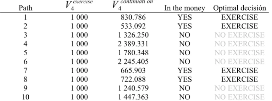
As with the binomial model, pinpointing the optimal exercise policy for the abandonment option entails applying a recursive optimisation process commencing at the option expiry date (t=4) and concluding at the first exercise date (t=2). At the option expiry date, the strategy which maximises the extended value of the investment involves exercising the option for the trajectories in the money, as if it were a European derivative. In the abandonment option, the trajectories in the money will obviously be those for which the liquidation value of the business is greater than the continuation value. The liquidation value of the business coincides with the exercise price of the option, 1,000 monetary units. The continuation value (value of the business when the option is not exercised) is the result of discounting the cash flows generated from the expiry date, shown in Table 3:

 

, 5

* , 5 ,

4 ,

4 r

V S F

V

on continuati

i i i

on continuati

i 

 

being  

r S F

V^continuati_i ^on _i ⁱ

* , 5 , 5 ,

5 

4 Using only ten simulations entails an error in approximation which can be reduced by increasing the number of trajectories. For a simulation of 200,000 trajectories, the current value of the business comes to 1,259.29 monetary units.

11

where subscript i refers to the i-th simulated trajectory.

The calculations corresponding to each of the trajectories simulated are shown in Table 4. The outcomes to emerge from the simulations in the example reveal that four of these trajectories are in the money when the option expires, the strategy which maximises the extended value of the investment being that which derives from the abandonment of the project for these trajectories.

As can be seen, analysing the exercise strategy at expiry using the LSM method is carried out by simply considering the derivative as if it were European. After doing this, and taking the initial series of ten simulated trajectories, estimation of the optimal frontier at the moments of possible exercise prior to expiry can commence.

Table 4 Trajectories in the money at the option expiry date Path V₄^exercise V₄^continuation In the money Optimal decisión

1 1 000 830.786 YES EXERCISE 2 1 000 533.092 YES EXERCISE 3 1 000 1 326.250 NO NO EXERCISE

4 1 000 2 389.331 NO NO EXERCISE 5 1 000 1 780.348 NO NO EXERCISE 6 1 000 2 245.405 NO NO EXERCISE

7 1 000 665.903 YES EXERCISE 8 1 000 722.088 YES EXERCISE 9 1 000 1 240.579 NO NO EXERCISE

10 1 000 1 447.363 NO NO EXERCISE

This is where the main differences between the LSM and binomial models emerge. Monte Carlo simulation generates the approximation corresponding to a trajectory at a given moment, assuming that its value at the previous moment is known. Taken independently, each trajectory thus offers a perfect foresight solution, simulation of a large number of trajectories proving necessary if a good approximation to the state variable is to be achieved. By contrast, at a given moment in the binomial model each value of the variable generates at least two possible scenarios in the following period.

In order to know what to do when faced with a specific trajectory at a specific point, procedures which use simulation in American options valuation require some kind of mechanism offering an expected exercise frontier.

In the LSM model, this is performed by statistical regression. Thus, at each point at

5Estimating the most suitable exercise strategy for each trajectory is not recommendable since the decision to exercise the option at a given point is taken assuming that the information from future moments is known, which yields an upwards biased value for the option.

12

which early exercise of the option is allowed, the continuation value or value of the investment when the option is going to be maintained until next period (dependent variable) is regressed on some transformations of the simulated value of the state variable (independent variables). Moreover, this regression is only posited for trajectories which are in the money at a specific point

, since, a priori, they are the only ones for which continuing the business is worth considering.

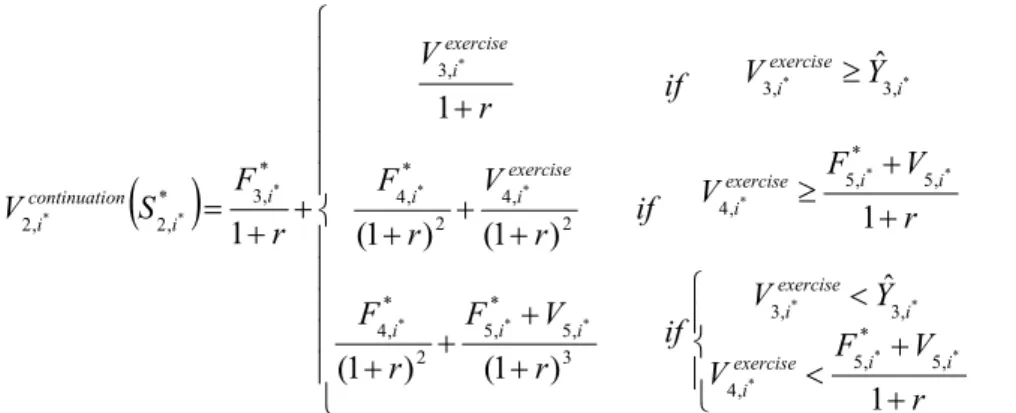
Below we show how the successive regressions of the investment in hand would be formulated. At t=3 the option holder must decide whether to exercise the option immediately, in other words, abandon the project, yielding a value of

monetary units, or to carry on to the next point, t=4, and opt for the wisest choice. The value of the latter possibility is obtained by applying the optimal exercise policy from t=4 which, as it coincides with expiry, involves comparing the values of the underlying investment if either exercising the option or not. The value of keeping the option alive at t=3 is thus given by:

 

















 



 





 

 

) 1 (

) 1 (

) 1 (

1 1

*

*

*

*

*

*

*

*

*

*

*

*

, 5

* , 5 ,

4

, 5

* , 5 ,

4

2 , 5

* , 5 , 4

* ,

* 4 , 3 ,

3

r V V F

r V V F

if if

r V F

r V r S F

V

i exercise i

i

i i exercise

i

i i

exercise i

i i on continuati

i

where the subscript i

represents the set of trajectories in the money at point

The continuation value thus obtained is the dependent regression variable,

. The independent regression variables are based on the simulated values of the state variable. For the purpose of illustration, we use a degree two polynomial regression,

the equation to be estimated at this point therefore being:

 

* , 3 3 3

* , 3 ,

3_i^* S _i^* a (S _i^*) S _i^*

Y  



 where

 

 

6 Trajectories in the money are those for which the value of the business if the option is exercised is greater than the value if it is not, as if expiry of the right were to occur at that point.

7As regards the basic functions to be used in regression, Longstaff and Schwartz (2001) and Moreno and Navas (2003) propose using up to a two degree polynomial function as a good approximation to the exercise frontier.

13

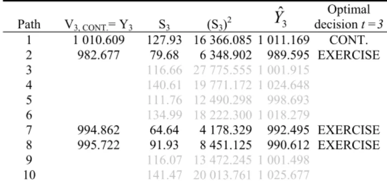
Table 5 shows the variables involved in the regression at t=3 for trajectories in the money at this point, which are trajectories 1, 2, 7 and 8. After analysing the optimal decision corresponding to these trajectories one period later, at t=4, the second column shows the

continuation values obtained from the future cash flow discount to emerge from optimal abandonment/non- abandonment. The following approximation coefficients are estimated from the vectors corresponding to the independent regression variables –columns three and four–,

2

* 3

* 3

3 1057.046 1.652 0.010( )

ˆ S S

Y   

Finally, columns five and six show the result of regression for trajectories in the money at t=3. The optimal decision reached for each trajectory at t=3 is obtained simply by comparing the continuation value derived from regression,

, and the liquidation value of the business, in other words 1,000 monetary units. As can be seen, the optimal decision at t=3 is immediate abandonment of the business for trajectories 2, 7 and 8, whereas for trajectory 1 the optimal decision is to continue with the business until at least t=4.

Table 5. Variables involved in regression at t = 3 Path V3, CONT.= Y3 S3 (S3)² Yˆ³ decision t =3 ^Optimal

1 1 010.609 127.93 16 366.085 1 011.169 CONT.

2 982.677 79.68 6 348.902 989.595 EXERCISE 3 116.66 27 775.555 1 001.915

4 140.61 19 771.172 1 024.648 5 111.76 12 490.298 998.693 6 134.99 18 222.300 1 018.279

7 994.862 64.64 4 178.329 992.495 EXERCISE 8 995.722 91.93 8 451.125 990.612 EXERCISE 9 116.07 13 472.245 1 001.498

10 141.47 20 013.761 1 025.677

The function of the expected continuation value for point t=2 is estimated

in the same way as for t=3. Determining the exercise policy entails regressing

the value of the project in the event of continuation over the constant and

simulated values of the only source of uncertainty considered. The continuation

values for trajectories in the money at t=2 are calculated applying the optimal

decisions calculated for the following moments, t=3 and t=4, in such a way that

exercising the option is considered as soon as the critical frontier is reached:

14

 



























 





 





 



 





 



r V V F

Y V

r V V F

Y V

if if

if

r V F r F

r V r F

r V

r S F

V

i i exercise

i

i exercise

i

i i exercise

i

i exercise

i

i i i

exercise i i

exercise i

i i on continuati

i

1 ˆ 1

ˆ

) 1 ( ) 1 (

) 1 ( ) 1 (

1

1

*

*

*

*

*

*

*

*

*

*

*

*

*

*

*

*

*

*

*

, 5

* , 5 ,

4

, 3 ,

3

, 5

* , 5 ,

4

, 3 ,

3

3 , 5

* , 5 2

* , 4

2 , 4 2

* , 4

, 3

* ,

* 3 , 2 ,

2

where, once again the subscript i

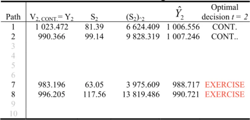
represents the trajectories in the money at point t=2, of the ten initial simulations. In t=2 trajectories 1, 2, 7 and 8 remain in the money.

As can be seen, the regression dependent variable,

, is calculated from the “real” values of the flows and not from the expected continuation value which is derived from the previously estimated regression.

Approximation of the expected function of the value of keeping the option alive at t=2 is given by the following expression:

2 2 2

2 794.556 4.711 0.026( )

ˆ S S

Y   

For point t=2, Table 6 shows the “real” values derived from continuing with the business at least up to the following period and the continuation values estimated from regression.

The optimal exercise strategy at t=2 is shown in the final column, abandonment of the business for trajectories 7 and 8 and continuation thereof for at least one more period for trajectories 1 and 2 proving the optimal course of action.

Table 6. Variables involved in regression at t = 2 Path V2, CONT.= Y2 S2 (S2)^2 Yˆ2 decision t = 2 ^Optimal

1 1 023.472 81.39 6 624.409 1 006.556 CONT.

2 990.366 99.14 9 828.319 1 007.246 CONT..

3 4 5 6

7 983.196 63.05 3 975.609 988.717 EXERCISE 8 996.205 117.56 13 819.486 990.721 EXERCISE 9

10

15

By applying the abandonment rule identified at each of the exercise opportunities evaluated, abandoning the business proves optimal for trajectories 7 and 8 at point t=2, for trajectory 2 at t=3, and for trajectory 1 at the expiry date

abandoning the business felt to be a recommendable course of action. By thus specifying the optimal exercise strategy, determining the cash flows to emerge from the most recommendable decisions for each case proves fairly straightforward. Table 7 shows the extended present value of the underlying investment project derived from the optimal decision in each case.

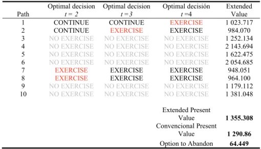
After averaging the outcomes obtained for each trajectory, we see how the value derived from active management of the underlying investment, the Extended Value, comes to 1,355.31 monetary units compared to the 1,290.86 monetary units which the traditional “passive” cash-flow discount of the project yields. The value of the option to abandon is therefore 64.45 monetary units.

Estimation of such a small number of trajectories is clearly insufficient to obtain a good approximation of the option value

. However, the Monte Carlo method allows us to enhance the quality of the approximation by increasing the number of simulations, as inversely the standard error of its estimation depends on the number of experiments performed, whatever the temporal dimension of the problem.

Table 7. Estimation of the Extended Value of the Investment Path Optimal decision

t = 2 Optimal decision

t =3 Optimal decisión

t =4 Extended

Value 1 CONTINUE CONTINUE EXERCISE 1 023.717 2 CONTINUE EXERCISE EXERCISE 984.070 3 NO EXERCISE NO EXERCISE NO EXERCISE 1 252.134 4 NO EXERCISE NO EXERCISE NO EXERCISE 2 143.694 5 NO EXERCISE NO EXERCISE NO EXERCISE 1 622.475 6 NO EXERCISE NO EXERCISE NO EXERCISE 2 054.685

7 EXERCISE EXERCISE EXERCISE 948.051

8 EXERCISE EXERCISE EXERCISE 964.100

9 NO EXERCISE NO EXERCISE NO EXERCISE 1 179.112 10 NO EXERCISE NO EXERCISE NO EXERCISE 1 381.048

Extended Present

Value 1 355.308 Convencional Present

Value 1 290.86 Option to Abandon 64.449

8 The fact that the number of simulations is extremely low causes the difference between the outcome of the valuation from the binomial model and that obtained through the LSM algorithm.

16 2.3. Comparing the binomial model and the LSM model

As can be seen, valuing the investment case posited proves more straightforward using the binomial model, since the initial hypotheses fit the assumptions on which the model is based very well. In fact, the assumption that the sources of uncertainty involved in the business may be summed up in a single variable –demand– stochastic evolution of which is approached using geometric Brownian movement, is established so as to facilitate the estimation of the upward and downward variations of the discretisation process. Moreover, simplification of the abandonment possibilities to a small number of dates allows implementation of the dynamic programming recursive procedure of the binomial model using a simple spreadsheet.

The LSM procedure merges information from the discretisation of the variable not only with dynamic programming but also statistical regression. This is because each trajectory generated using the Monte Carlo method constitutes a perfect foresight solution, making necessary both simulation of a large number of trajectories as well as use of some technique to provide an expected stopping at the correct approximation of the value option.

From the above it can be deduced that implementing the LSM procedure proves a priori less intuitive and more complex than the binomial model, as a result of which its use depends on the possibilities of applying the latter.

Common factors such as an increase in the number of exercise dates, the existence of multiple sources of uncertainty or adjusting its future evolution to patterns other than Brownian, complicate application of the binomial model, when indeed not rendering it impossible.

One example is that including a second stochastic factor entails a

substantial alteration of the tree shape representation which the procedure

adopts. In addition to the joint density of the two variables needing to follow a

bivariate lognormal distribution, the discrete approximation of the two variables

needs to be constructed based on a five node scheme, giving rise to a three

dimensional tree in the shape of an inverted pyramid. Extending this

representation to the subintervals into which the valuation period is divided

means exponentially increasing the possible states of the nature, complicating

17

implementation of the recursive process required to estimate the optimal stopping rule.

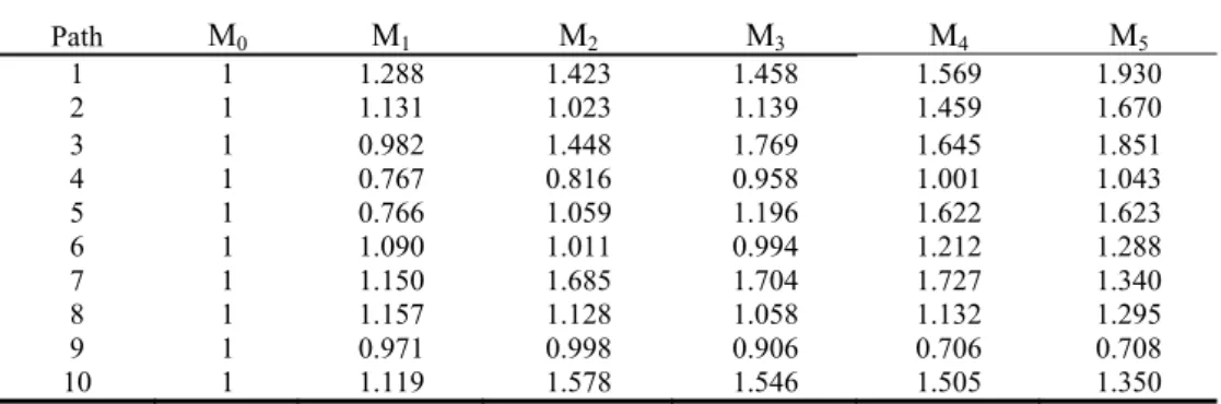
For its part, in the LSM method, including a second stochastic factor merely involves doubling the effort required for initial simulation of the state variables and extending the number of independent variables involved in regression. However, it does not entail any change in the method applied to estimate the exercise frontier linked to possible abandonment. For example, if

= 6%, σ

= 15% and μ

= 6%, not correlated

with the evolution of the first stochastic factor, we would only need to generate the sample representations corresponding to the second variable, shown in Table 8, and obtain, together with those corresponding to the first stochastic factor, the net cash flows of the project as shown in Table 9.

Table 8. Second factor stochastic simulations throughout the lifespan of the investment

Table 9. Estimated flows throughout the lifespan of the investment

Path F1 F2 F3 F4 F5 V5

1 79.066 57.980 93.341 95.898 80.245 1 603.105 2 48.406 50.785 45.425 46.427 44.572 890.434 3 51.221 74.863 103.306 127.343 122.895 2 455.140 4 34.245 45.115 67.457 81.549 124.680 2 490.810 5 50.813 80.167 66.887 80.469 144.613 2 889.024 6 88.220 70.490 67.189 126.339 144.734 2 891.432 7 49.517 53.187 55.151 77.015 44.651 892.021 8 69.356 66.379 48.666 51.510 46.796 934.8634 9 50.131 59.146 52.626 46.813 43.955 878.118 10 71.164 108.955 109.479 121.669 97.829 1 954.392 Average 59.214 66.707 70.953 85.503 89.497 1 787.934

9 In order to simplify the explanation, we assume the same process used for modelling the first stochastic factor.

Thus, we can use the same expressions presented previously to the margin simulation, with simple replacement of the values of their parameters.

10 See Alonso (2007) for simulation of random correlated variables.

Path M0 M1 M2 M3 M4 M5

1 1 1.288 1.423 1.458 1.569 1.930 2 1 1.131 1.023 1.139 1.459 1.670 3 1 0.982 1.448 1.769 1.645 1.851 4 1 0.767 0.816 0.958 1.001 1.043 5 1 0.766 1.059 1.196 1.622 1.623 6 1 1.090 1.011 0.994 1.212 1.288 7 1 1.150 1.685 1.704 1.727 1.340 8 1 1.157 1.128 1.058 1.132 1.295 9 1 0.971 0.998 0.906 0.706 0.708 10 1 1.119 1.578 1.546 1.505 1.350

18

Based on the values of the cash-flows, implementing the LSM method to estimate the Extended Present Value of the business involves the same operations routine as in the case of a stochastic factor. We simply need to include the terms of the second stochastic factor together with the crossed product of the sources of uncertainty in the series of independent variables in regression. In this case, the abandonment option comes to 40.71 monetary units.

3. Conclusion

New valuation proposals based on Monte Carlo simulation, dynamic programming and statistical regression are destined to revolutionise business valuation and business investments. These flexible models are able to value different sources of value in any kind of investment regardless of the nature of its options and sources of uncertainty. In this vein and in just a short space of time, the algorithm proposed by Longstaff and Schwartz (2001) has emerged as the procedure for valuing American, financial or real derivatives to have the greatest practical impact. The growing number of papers, prominent amongst which are Schwartz and Moon (2000 and 2001), Miltersen and Schwartz (2004), Schwartz (2004), Gravet (2003), León and Piñeiro (2004), Rubio and Lamothe (2006), Abadie and Chamorro (2006) and Alonso, Azofra and Fuente (2009) to name but a few, bear witness to its possibilities for development and adaptation to business investment and options.

The LSM algorithm is the result of merging three different techniques, each of which contributes its own advantages to the valuation procedure.

Firstly, Monte Carlo simulation greatly extends the range of possible stochastic processes to be considered when characterising sources of uncertainty.

Secondly, dynamic programming allows the possibility of early exercise in the

valuation of American style options to be included, and thirdly, statistical

regression allows the calculation problem involved in valuing options dependent

on multiple sources of uncertainty to be solved. Overall, the LSM algorithm

provides a flexible and powerful tool capable of valuing virtually any kind of

option using up only a limited amount of resources.

19

The main drawback of this procedure lies in the fact that its application requires a high degree of calculation, which is only assumable through an automated software package. The use of these valuation packages by those in charge of financial management may entail a certain loss in transparency as far as the calculation process is concerned. For this reason, it is interesting to shed some light on the “black box” of this kind of optimisation tool and to facilitate understanding of the principles governing its functioning.

Nevertheless, the search for flexibility in valuation models is justified

whenever the benefits in terms of greater accuracy and operational simplicity of

the valuation, make up for the costs in terms of abstraction and implementation

of the new proposals. Specifically, when the option valued may be exercised at

various points prior to the expiry date, its value depends on multiple sources of

uncertainty or if the latter follow stochastic processes other than Brownian, the

LSM model which we have explained here emerges as the most efficient of the

existing alternatives.

20

References

Abadie, L. M., Chamorro, J. M., 2006. Valuation of Natural Gas Power Plant Investment. Presented at the X Real Options Conference, New York.

Alonso, S.; Azofra, V.; Fuente, G. de la, 2009. Las opciones reales en el sector eléctrico. El caso de la expansión de Endesa en Latinoamérica. Cuadernos de Economía y Dirección de la Empresa, 38, 65-94.

Amram, M., Kulatilaka, N., 1999. Real Options: Managing Strategic Investment in an Uncertainty World. Harvard Business School Publications.

Aggarwal, R., 1993. Capital Budgeting under Uncertainty, Prentice-Hall, Englewood Cliffs, New Jersey.

Copeland, T., Tufano, P., 2004. Las opciones reales y su gestión en el mundo real.

Harvard-Deusto Business Review, 82 (3), 86-96.

Cox, J. C.; Ross, S. A.; Rubinstein, M., 1979. Option Pricing: A Simplified Approach.

Journal of Financial Economics, 7, 229-263.

Gravet, M. A., 2003. Evaluación de opciones reales mediante simulación: El método de los mínimos cuadrados. Memoria para optar al título de Ingeniero Civil Industrial.

Pontificia Universidad Católica de Chile, Santiago de Chile.

Lander, D., Pinches, G., 1998. Challenges to the Practical Implementation of Modeling and Valuing Real Options, Quarterly Review of Economics and Finance, 38, 537- 567.

León, A., Piñeiro, D., 2004. Valuation of a biotech company: A real options approach, Working paper CEMFI.

Longstaff, F. A., Schwartz, E. S., 2001. Valuing American Options by Simulation: A Simple Least-Squares Approach. The Review of Financial Studies, 14 (1), 113- 147.

Miltersen, K. R., Schwartz, E. S., 2004. R&D Investments with Competitive Interactions. Review of Finance, 8, 355–401.

Moreno, M., Navas, J. F., 2003b. On the Robustness of Least-Squares Monte Carlo (LSM) for Pricing American Derivatives. Review of Derivatives Research, 6 (2), 107-128.

Myers, S. C., 1977. Determinants of Corporate Borrowing, Journal of Financial Economics, 5, 147-175.

Myers, S. C., 1996. Fischer Black´s Contributions to Corporate Finance, Financial Management, 25 (4), 95-103.

Newton, D. P., Pearson, A. W., 1994. Application of OPT to R&D, R&D Management, 24 (1), 83-89.

Rubio, G., Lamothe, P., 2006. Real Options in Firm Valuation: Empirical Evidence from European Biotech Firms. Presented at the X Real Options Conference, New York.

21 Schwartz, E. S., 2004. Patents and R&D as Real Options”, Economics Notes, 33, 1,

23-54.

Schwartz, E. S., Moon, M., 2000. Rational Pricing of Internet Companies, Financial Analyst Journal, 56 (3), 62-75.

Schwartz, E. S., Moon, M., 2001. Rational Pricing of Internet Companies Revisited, Financial Review, 36, 7-26.

F

C

A

Últimos números publicados

159/2000 Participación privada en la construcción y explotación de carreteras de peaje Ginés de Rus, Manuel Romero y Lourdes Trujillo

160/2000 Errores y posibles soluciones en la aplicación del Value at Risk Mariano González Sánchez

161/2000 Tax neutrality on saving assets. The spahish case before and after the tax reform Cristina Ruza y de Paz-Curbera

162/2000 Private rates of return to human capital in Spain: new evidence F. Barceinas, J. Oliver-Alonso, J.L. Raymond y J.L. Roig-Sabaté 163/2000 El control interno del riesgo. Una propuesta de sistema de límites

riesgo neutral

Mariano González Sánchez

164/2001 La evolución de las políticas de gasto de las Administraciones Públicas en los años 90 Alfonso Utrilla de la Hoz y Carmen Pérez Esparrells

165/2001 Bank cost efficiency and output specification Emili Tortosa-Ausina

166/2001 Recent trends in Spanish income distribution: A robust picture of falling income inequality Josep Oliver-Alonso, Xavier Ramos y José Luis Raymond-Bara

167/2001 Efectos redistributivos y sobre el bienestar social del tratamiento de las cargas familiares en el nuevo IRPF

Nuria Badenes Plá, Julio López Laborda, Jorge Onrubia Fernández

168/2001 The Effects of Bank Debt on Financial Structure of Small and Medium Firms in some Euro- pean Countries

Mónica Melle-Hernández

169/2001 La política de cohesión de la UE ampliada: la perspectiva de España Ismael Sanz Labrador

170/2002 Riesgo de liquidez de Mercado Mariano González Sánchez

171/2002 Los costes de administración para el afiliado en los sistemas de pensiones basados en cuentas de capitalización individual: medida y comparación internacional.

José Enrique Devesa Carpio, Rosa Rodríguez Barrera, Carlos Vidal Meliá

172/2002 La encuesta continua de presupuestos familiares (1985-1996): descripción, representatividad y propuestas de metodología para la explotación de la información de los ingresos y el gasto.

Llorenc Pou, Joaquín Alegre

173/2002 Modelos paramétricos y no paramétricos en problemas de concesión de tarjetas de credito.

Rosa Puertas, María Bonilla, Ignacio Olmeda

174/2002 Mercado único, comercio intra-industrial y costes de ajuste en las manufacturas españolas.

José Vicente Blanes Cristóbal

175/2003 La Administración tributaria en España. Un análisis de la gestión a través de los ingresos y de los gastos.

Juan de Dios Jiménez Aguilera, Pedro Enrique Barrilao González

176/2003 The Falling Share of Cash Payments in Spain.

Santiago Carbó Valverde, Rafael López del Paso, David B. Humphrey Publicado en “Moneda y Crédito” nº 217, pags. 167-189.

177/2003 Effects of ATMs and Electronic Payments on Banking Costs: The Spanish Case.

Santiago Carbó Valverde, Rafael López del Paso, David B. Humphrey

178/2003 Factors explaining the interest margin in the banking sectors of the European Union.

Joaquín Maudos y Juan Fernández Guevara

179/2003 Los planes de stock options para directivos y consejeros y su valoración por el mercado de valores en España.

Mónica Melle Hernández

180/2003 Ownership and Performance in Europe and US Banking – A comparison of Commercial, Co- operative & Savings Banks.

Yener Altunbas, Santiago Carbó y Phil Molyneux

181/2003 The Euro effect on the integration of the European stock markets.

Mónica Melle Hernández

182/2004 In search of complementarity in the innovation strategy: international R&D and external knowledge acquisition.

Bruno Cassiman, Reinhilde Veugelers

183/2004 Fijación de precios en el sector público: una aplicación para el servicio municipal de sumi- nistro de agua.

Mª Ángeles García Valiñas

184/2004 Estimación de la economía sumergida es España: un modelo estructural de variables latentes.

Ángel Alañón Pardo, Miguel Gómez de Antonio

185/2004 Causas políticas y consecuencias sociales de la corrupción.

Joan Oriol Prats Cabrera

186/2004 Loan bankers’ decisions and sensitivity to the audit report using the belief revision model.

Andrés Guiral Contreras and José A. Gonzalo Angulo

187/2004 El modelo de Black, Derman y Toy en la práctica. Aplicación al mercado español.

Marta Tolentino García-Abadillo y Antonio Díaz Pérez 188/2004 Does market competition make banks perform well?.

Mónica Melle

189/2004 Efficiency differences among banks: external, technical, internal, and managerial Santiago Carbó Valverde, David B. Humphrey y Rafael López del Paso

190/2004 Una aproximación al análisis de los costes de la esquizofrenia en españa: los modelos jerár- quicos bayesianos

F. J. Vázquez-Polo, M. A. Negrín, J. M. Cavasés, E. Sánchez y grupo RIRAG 191/2004 Environmental proactivity and business performance: an empirical analysis

Javier González-Benito y Óscar González-Benito

192/2004 Economic risk to beneficiaries in notional defined contribut