1995-2013
A STOCHASTIC ANALYSIS
José Luis Rojas Aguilar Fernando Sánchez Vera
Instituto Tecnológico y de Estudios Superiores de Monterrey
DR. JOSÉ LUIS ROJAS AGUILAR DR. FERNANDO SÁNCHEZ VERA
Researcher at ITESM campus Chiapas. Contact: [email protected] Researcher at ITESM. Contact: [email protected]
ABSTRAC
This article seeks to model the new theories of multidimensional poverty measurement. The proposed model considers the poverty of capabilities and poverty of needs as complementary and not as substitutes (Discussed extensively in the literature on the subject) consistent with new currents that support a multifactorial definition.
Through a stochastic model the breaking of the traditional paradigm of measuring poverty indicators is sought with Static and deterministic models, at the same time providing a dynamic picture of the evolution of poverty, which has a historical memory in its formation. This model is applied to the various dimensions of poverty through income in Mexico discriminating between rural and urban areas.
Keywords: Evolution of poverty, social mobility, social heterogeneity, Transition probability, Markov Chains, multidimensional poverty in Mexico.
I
n order to study the evolution of the structure of poverty and examine the characteristics of the process of social mobility between the different dimensions of income poverty in Mexico, this article has considered the following: the evolution of poverty is a dynamic process of mobility between different dimensions of income that affect humans, food poverty, capacity and capital. It is assumed that people are constantly looking to improve their income and change their living conditions. Also, mobility takes place in a space open to opportunities through the creation and discovery of new strategies for the formation of human capital, their entry into the market and their sustainability in the long term. It is understood that there is heterogeneity in access and utilization of social programs, due to:a. The space of poverty is complex and multidimensional;
b. That society is experiencing social and economic change;
c. That the poor population is heterogeneous in its needs and wants;
d. That different social conditions coexist that lead to differing degrees of success and failure in the formation of human capital, poverty alleviation and development.
The relative success or failure of social policies in the process of evolution of poverty can be measured in terms of the transition probability of overcoming a dimension or to move to a dimension of higher income.
De esto trata el presente texto: del uso de las estrategias usadas por los candidatos en las elecciones referidas, haciendo énfasis en aquellas que recurrieron a la estimulación de las emociones, a través del miedo y la comedia.
1 It is assumed that the State or NGOs continue strategic routines through actions and programs to increase social capital and human development of the population, and the review of these strategies is directly linked to their success.
THE PROBABILITIES OF POVERTY
Each transition probability is the probability that a person in poverty i at time t is exceeded and goes on to the next dimension j poverty in which their deficiencies decrease at time t + 1. If i = j then the transition probability becomes an indicator of the inability of people to overcome their poverty from one period to another. If i ≠ j then the transition probability can be interpreted as the relative mobility of poverty dimensional j in the attraction of dimension i. A stochastic Markov process of first order is assumed.
The probability distribution for mobility from one dimension to another population is conditioned to its previous size. Therefore, each transition probability is conditional on the size of the population in the previous period, so you can make the following transition probability matrix:
If there is a fragmentation of mobility, or lack of social mobility between the dimensions of poverty, it will be reflected in the matrix of transition probabilities. The matrix also shows whether the mobility process is more intense.
The transition probabilities are described as the proportion of the population who are in any of the dimensions of income poverty and changing to another dimension over time. Consequently, they become the parameter of the equations of motion of the social structure.
STOCHASTIC MODELS TO EXPLAIN THE EVOLUTION OF POVERTY
Poverty, either for its causes (psychological, social, economic, political ...) is a complex and multifactorial phenomenon that when combined,
results in states other than the social condition of the individual (food poverty, capabilities, non-vulnerable assets) . This presents stochastic elements and makes known the limitations of deterministic models to explain measure and compare culturally heterogeneous groups over time. People perform different actions and strategies (for example, modify their consumption, expand their job skills, training, etc.) and divergent behaviors in different social groups has been observed within different economic scenarios (recession, stability or growth) thereby the result of thier social status given their actions and strategies should be modeled as a stochastic outcome, given the complexity required a multifactorial model is proposed and the inability to model the heterogeneity that is posed by various social groups.
Stochastic models have been commonly used in the analysis of social statistics to model the evolution of populations4. The obligatory stochastic reference models are Gibrat’s Law of Proportionate growth5. He uses a stochastic approach to model the evolution of the distribution of the population in a sector with a number of control groups where:
a. Growth rates of each population group are stochastic, with a probability distribution that can be specified (usually normality is assumed).
b. The probability distribution for growth rates of population groups are independent of the size of the community.
c. and that the probability distribution is independent of the past history of population growth.
This very simple stochastic model is able to describe (and perhaps explain) the behavior of the concentration in many populations6.
4 For example Rothblum and Winter (1985), Ijiri and Simon (1977) and the pioneering work of Hart and Prais (1956).
Scherer and Ross (1990), pp 141-146, contains a good introduction to the literature on stochastic growth model.
5 Gibrat (1931).
6 See Seherer and Rose (1990), pp 141-146.
MODELS BASED ON THE BEHAVIOR OF STOCHASTIC POPULATION MODELS
Some authors argue 7 that there is some stochastic element in the nature of human beings and in particular their behavior when making a decision.
Consequently, stochastic models of population behavior are very popular in the research of consumer behavior in economic literature.
This section explains the underlying model, under the assumption of the heterogeneity of poverty, assuming that:
a. There are options that a person can have different states of poverty (food, capacities, assets, and non-vulnerable) among different groups of the population.
b. The position of being poor at birth of a person is defined stochastically in terms of a vector of probabilities of θ (t) = [∅_ (1) (t), ∅_2 (t), ... ∅_ (n) (t )], where ∅_ (i) (t) refers to the probability that a person is in a degree of poverty at time t.8 c. The probability distribution vector is independent of the
previous actions of the person (zero-order model).
The probability distribution of ∅ (t) indicates that the person has a stochastic behavior, but the specific distribution of ∅ (t) is determined by two factors: the initial conditions of individuals at birth and secondly, the cultural, social and economic conditions of their society.
The initial condition defines absolute poverty, in terms of the attributes of the individual’s family and the person is determined as poor in relative terms with the options available in their community9. The second states that this behavior plays an important role in determining
7 See Bass (1974), Bass and Pilon (1980), Lipstein (1965), Massy (1970), and Lilien (1992), Red (1993).
8 The model assumes that each individual will suffer to the same extent from the lack or deficiency that is measured in terms of income.
9 See Lancaster (1996).
their future poverty status thus modifying its multidimensional space.10 A person is considered successful if i can improve their conditions (income, health, education, heritage, etc.) so that ∅_ (i) (t) is greater than anywhere ∅_ (j) (t).
If individuals are heterogeneous in their conditions, and it is possible to define m different groups and each group consists of members q, the probability distribution for the condition of poverty is different between groups. Mathematically, the vector ^ q ∅ (t ) is a specific group, the new specification is ∅ ^ q (t) = [∅_1 ^ q (t), ..., ^ ∅_n q (t)]; , And q = 1, ..., m; where ∅_i ^ q (t) is the probability that a person in a condition of type q poverty will go on to type i poverty group at time t.
Then, you can define the conditional probabilities Pij, which indicate the average probability for a person in poverty dimension j at time t. The transition probability is given as follows:
Where i, j = 1,2, ... n
Taking into account the n conditions of poverty of the individual, in (nxn) the matrix of transition probabilities is defined.
Taking into account the transition probabilities Pij and supposing that they are stationary and the number of people that are found in the state of poverty known at the moment t, then it is possible to calculate the expected number of the people in state of poverty in the period t+ 1.
Where S(t) is the total number of people in society at moment t, and if S_i(t)
10 See Capozza and Van Order (1978), Schmalensee (1978), Moorthy (1988), Hauser (1988), and Shaked and Sutton (1982). The pioneer in localization models (1929). Ver Lilien (1992), Chapter 5.
Is the total number of people in the state of poverty I at moment t:
Where the vector describing the distribution of individuals among the different dimensions of poverty at time t which can be defined:
[S_1 (t), S_2 (t), ..., S_in (t)]. The expected number of people in poverty dimension j at time t + 1 is given by the following formula, which describes a stochastic Markov process of first order for the group of people in society:
Therefore, if the behavior of the family is characterized by a stochastic process of a zero order and if there is heterogeneity in the characteristics of poverty, the first Markov stochastic order process reflects the evolution of the aggregate of individuals (number of poor in dimension j) describing the behavior of the switched dimension of its origin.
In general, it is assumed that there is no entry of new people. In this case S_i (t) = S_ (t-1), and the process described in equation (4) can be expressed in terms of the total proportion of the population of society if we divide both sides of the equation by S_ (t). Thus, a first order process describes the evolution of the different dimensions of poverty.
a. People born into poverty have the behavior from their family and social group initially specified, described by equation (4).
b. The different dimensions of poverty attract new people at the same rate as those new people who are born into it. Therefore, let N (t) as the total number of new poor in period and N_j (t) is the total number of new people born in dimension j at time t. Therefore, this assumption implies:
The course leads to the equation (5) which simplifies the analysis and is justified because it seems reasonable to assume that births and immigration to the dimension of poverty must be correlated with the ability of that dimension for retaining people, Therefore, the dimension size (number of people in food poverty, skills or equity) is described by the following equation:
If we manipulate the equation (6) it leads to the following process describing the evolution of the size of the dimension of poverty:
This implies the following stochastic process underlying the first order which characterizes the evolution of the proportions of each dimension of poverty when people are heterogeneous and behave
according to a stochastic process of zero order, and / or new births and immigration of people which is represented by the equation:
MARKOV STOCHASTIC PROCESSIN THE EVOLUTION OF POVERTY IN MEXICO
The use of a first order stochastic Markov process is used to explain the evolution of poverty in Mexico, and implies that the actions and efforts made in the past stochastically influence on social mobility and the present development of families, based on families that take action (search for government and private support) to improve their human capital and will succeed if the proportion of people who are in the dimension j of poverty is reduced.
∅_j = (t): expresses the probability that a person who is located in the dimension j at time t, and Pij: expresses the probability that the person transits from one dimension of poverty to another or exceeds the period t-1 at time t.
The following system of n equations relates the probability ∅_j over time:
It is possible to express this system of equations in the metrical form as
In matrix notation, the equation becomes:
Where ∅ (t) is an n-dimensional vector of state probabilities, and P is a matrix n by n of the transition probabilities P_ij. Where each dimension of poverty is mutually exclusive and gated, the following two equations hold for each period:
The following paragraphs explain how the transition probabilities of a first order Markov process can be estimated using aggregate data showing the proportion of people in each of the different dimensions of income poverty in each period time. For a fuller explanation, see MacRae (1977), Lee (1970) and Rojas (1993).
A particular specification for the transition probabilities should be done since it is necessary to meet the following restrictions:
MacRae proposes the use of a multinomial logic formulation as suggested by Thai (1969). This formulation expresses the probability ratio as a function of an exogenous parameter11. Using the transition probabilities compared to the last column of the matrix P as the denominator, and since there are n columns in P, then the following relationships are formed (n-1 times):
The equation implies:
Adding through j = 1, ..., n
From equation (22) the following specification of the transition probabilities of the last elements of each column is obtained:
11 In this dissertation, the state assumes stationary transition probabilities. MacRae (1977) and others have sugges- ted the use of a variation in considering non-stationary states of the transition probability. In this case the transition probabilities are assumed as dependent on a set of explanatory variables.
Finally, equation (23) and (20) gives the following specifications for the other transition probabilities:
This specification of the transition probabilities implies that the system of equations in which the process of the first order Markov stochastic can be described as:
The equations (21) are very useful for estimation purposes. The transition probabilities are estimated indirectly, through direct parameter estimation β_ij. The specification of transition probabilities ensures its estimation so that this probability is not negative and the sum of the rows is equal to the unit. The equation system becomes a system of nonlinear equations.
SOCIAL MOBILITY BETWEEN URBAN AND RURAL AREAS IN MEXICO
In order to study social mobility among families of Mexican urban and rural areas, two matrices of transition probabilities were estimated. The estimation uses monthly data from 1995 to 2013, which includes the four dimensions of social mobility of lower income populations in Mexico.
It is useful to discriminate the poverty analysis spatially, dividing the population living in an urban (more than 25 thousand inhabitants) and rural (less than 25,000 inhabitants) zones in order to observe the structural change that occurs in the social sector of the country.
The study was restricted to four dimensions of income poverty;
it is observed that most of the elements of the diagonal are relatively
high. With values above 70 per cent and in the case of asset poverty, the likelihood of retention is higher. This information supports the claim that social mobility is very low and that the structure of poverty is not in balance.
The structure follows a path toward a stationary or immovable point (steady state condition), which is not stable and will probably never be achieved due to the forces of structural modification of both cyclical factors such as poverty. Therefore, the dimensions of poverty (tautological) are structures that are in a state of constant imbalance moving towards a long term dynamic equilibrium.
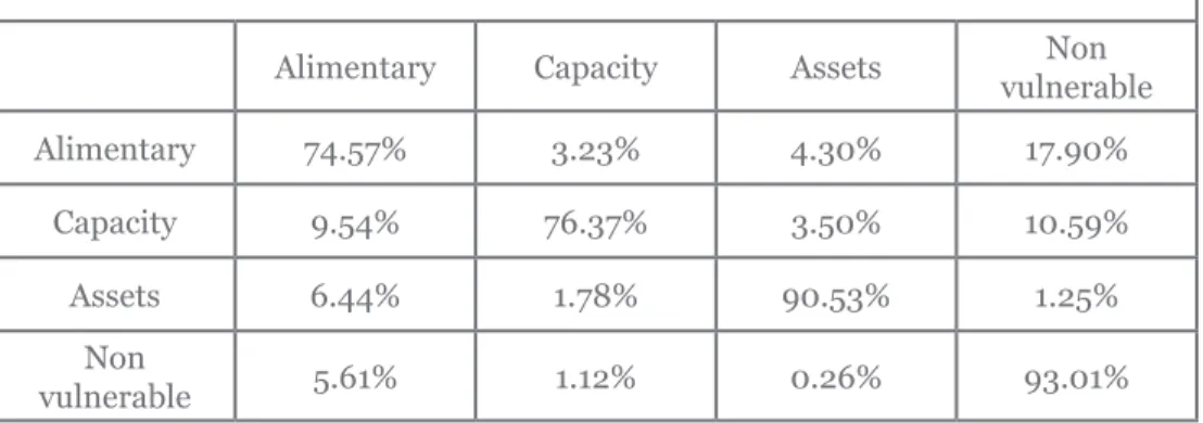
Table 1. Probability matrix of the transition of urban poverty in Mexico January 1995-December 2013
Alimentary Capacity Assets Non
vulnerable
Alimentary 74.57% 3.23% 4.30% 17.90%
Capacity 9.54% 76.37% 3.50% 10.59%
Assets 6.44% 1.78% 90.53% 1.25%
vulnerableNon 5.61% 1.12% 0.26% 93.01%
Source: Own estimation with data from CONEVAL 2013.
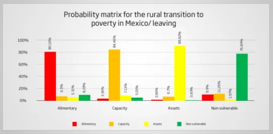
Table 2. Probability matrix of the transition of rural poverty in Mexico January 1995-December 2013
Alimentary Capacity Assets Non
vulnerable
Alimentary 83.41% 2.96% 2.54% 11.09%
Capacity 6.56% 74.37% 6.41% 12.66%
Assets 5.53% 6.28% 85.99% 2.21%
vulnerableNon 8.64% 4.45% 0.79% 86.13%
Source: Own estimation with data from CONEVAL 2013.
Tables 1 and 2 show that some transition probabilities outside the diagonal are close to zero, which shows a fragmentation of social mobility climbing with income and that the dimensions with higher population mass attracts more strongly the dimensions of lower mass. Poverty is higher in rural areas than in urban areas and food poverty has a high value for both matrices. However this condition has a relatively high rate of conversion that must be overcome by the official government programs.
The odds decrease, if the person is located in an urban area, but both parents have significantly higher elements on the main diagonal which indicates low social mobility.
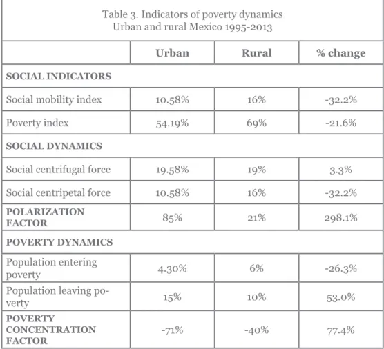
Table 3. Indicators of poverty dynamics Urban and rural Mexico 1995-2013
Urban Rural % change
SOCIAL INDICATORS
Social mobility index 10.58% 16% -32.2%
Poverty index 54.19% 69% -21.6%
SOCIAL DYNAMICS
Social centrifugal force 19.58% 19% 3.3%
Social centripetal force 10.58% 16% -32.2%
POLARIZATION
FACTOR 85% 21% 298.1%
POVERTY DYNAMICS Population entering
poverty 4.30% 6% -26.3%
Population leaving po-
verty 15% 10% 53.0%
POVERTY
CONCENTRATION
FACTOR -71% -40% 77.4%
Source: Own estimation with data from CONEVAL 2013.
Mobility was 32% higher in rural areas than in urban areas and income poverty was 21% more likely in rural areas. The expulsion of rural areas is 32% more likely than urban areas. There is a 26% chance of falling into poverty if you live in a rural area and 53% percent chance of overcoming income poverty if you live in an urban area.
In analyzing the dynamics of poverty, we can see that there was a strong trend towards urbanization of the population where people sought more developed urban communities or locations with urban conditions, the population concentrated with a 85% chance in an urban area and during the period a family living in an urban area had a 75%
chance of overcoming poverty and only a 40% chance if they lived in a rural area.
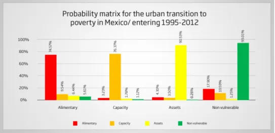
As we can see in Figure 1, social mobility is reduced and becomes stable to the extent that families migrate to urban areas, and the hypothesis that the retention capacity depends on the population mass that accounts for the size is met. The asset poverty was the dimension that attracted more families and expelled least within this period, so we can demonstrate that economic instability impacts more on income generating greater gateway to the entrance of poverty.
Graph 1. Probability matrix Urban and rural 1995-2012
Source: Own estimation with data from CONEVAL 2013.
Source: Own estimation with data from CONEVAL 2013.
MATRIX OF LONG TERM SOCIAL TRANSITION BETWEEN URBAN ZONES
Table 4. Stable state of long term probability of urban poverty in Mexico 1995-2012
State Name State Probability Recurrence Time
State 1 0.19 5.20
State 2 0.07 15.34
State 3 0.13 7.80
State 4 0.61 1.63
Expected Cost/Return= 0
Source: Own estimation with data from CONEVAL 2013.
The probabilities (Table 4) long-term studies show that the chances of being vulnerable are the highest in the dimensions of social mobility with 61% and the poverty of capabilities is the one with the lowest, probability according to the recurrence over time shows that it is easier to overcome poverty and harder to stay in capability poverty because once the dimension is exceeded, the possibility of return is almost 15
months, the size of non-vulnerable shows lower recurrence where only takes 2 months to return to the dimension.
Living in an urban area has high potential for overcoming poverty in the long-term health conditions and education are covered more effectively in the area, the food poverty would be the condition which affects most to urban areas this would affect 20% of the population.
Matrix of social transition between rural long term.
Table 4. Stable state of long term probability of urban poverty in Mexico 1995-2012
State Name State Probability Recurrence Time
State 1 0.19 5.20
State 2 0.07 15.34
State 3 0.13 7.80
State 4 0.61 1.63
Expected Cost/Return= 0
Source: Own estimation with data from CONEVAL 2013.
The long-term probabilities show that the chances of being vulnerable are reduced for inhabitants of rural areas and the probabilities are distributed homogenously between capacity poverty and asset poverty with 14% having the greatest vulnerability, as well as a dramatic reduction of food poverty.
We can say that urban conditions are an important factor in overcoming poverty but food poverty is a common denominator that it found in both areas, which requires actions and programs that can overcome this deficiency in the long term.
CONCLUSION
• The transition probabilities show the complexity of the social mobility of people in poverty.
• The probabilities fit the definition and design of multidimensional poverty, through a limited rationality and the incorporation of uncertain elements affecting poverty.
• The probabilities are adjusted to the complexity of the heterogeneity of the needs of the population with a stochastic and non-deterministic behavior.
• The probabilities capture the unsystematic risks of social development and changes in the macroeconomic and political environment.
• The high values of the main diagonal of the matrix of transition probabilities demonstrate the difficulty of the population in poverty, which is associated with involution of social capital, the disparity in economic growth of social groups, macroeconomic deterioration, inefficient and / or ineffective policies and actions of social actors (government, society and business).
• The near-zero off-diagonal values showed a scale pattern of social mobility, where the transition probability is reduced to the extent that it is further from its size. In other words, it is more likely to go from food poverty to capacity poverty than food poverty to not be vulnerable.
• The dimensions with the highest population mass attract more strongly than the dimensions of lower-mass population.
• One can see that the odds of being poor decreases if the person is located in an urban area, but both matrices presented low social mobility for Mexico in the period of 1995-2013.
• Social mobility was 32% higher in rural areas than in urban areas in the same period.
• Income poverty is 21% more likely in rural areas, and mobility in rural areas is 32% more likely than in an urban area.
• The population is concentrated with an 85% probability in an urban area, where a family living in an urban area had a 75% chance of overcoming poverty compared to 40% of the population living in a rural area.
• We can say that the conditions of civility represent an important factor in overcoming poverty, but food poverty is a common denominator that occurs in both areas, which requires actions and programs that can overcome this deficiency in the long term.
• The odds of falling into poverty are higher than those to overcome it, so we can conclude that the door to poverty is wider than its exit during this period.