MERCURY CONCENTRATION ACROSS A GRADIENT OF FOOD WEB COMPLEXITY AND ENVIRONMENTAL VARIABLES
by
Montana Gilbert
FACULTY OF NATURAL RESOURCES MANAGEMENT LAKEHEAD UNIVERSITY
THUNDER BAY, ONTARIO
April 2023
COMPLEXITY AND ENVIRONMENTAL VARIABLES
by
Montana Gilbert 1098868
An Undergraduate Thesis Submitted in Partial Fulfillment of the Requirements for the Degree of Honours Bachelor of Environmental Management
Faculty of Natural Resources Management Lakehead University
April 2023
--- ---
Dr. Brian McLaren Mr. Alex Ross
Major Advisor Second Reader
LIBRARY RIGHTS STATEMENT
In presenting this thesis in partial fulfillment of the requirements for the HBEM degree at Lakehead University in Thunder Bay, I agree that the University will make it freely available for inspection.
This thesis is made available by my authority solely for the purpose of private study and may not be copied or reproduced in whole or in part (except as permitted by the Copyright Laws) without my written authority.
Signature:____________________________
Date:____________________________
A CAUTION TO THE READER
This HBEM thesis has been through a semi-formal process of review and
comment by at least two faculty members. It is made available for loan by the Faculty of Natural Resources Management for the purpose of advancing the practice of
professional and scientific forestry.
The reader should be aware that opinions and conclusions expressed in this document are those of the student and do not necessarily reflect the opinions of the thesis supervisor, the faculty, or of Lakehead University.
ABSTRACT
Gilbert, M.K. 2023. Assessment of lake trout (Salvelinus namaycush) mercury concentration across a gradient of food web complexity and environmental variables. 56 pp.
Keywords: aquatic ecology, bioaccumulation, food chain length, freshwater fisheries lake class, lake trout (Salvelinus namaycush), mercury concentration
Exposure to mercury has been linked to health risks in both people and wildlife.
In Ontario, mercury pollution is to blame for 85% of the consumption restrictions on fish from inland lakes. Heavy metals like mercury accumulate up the food chain.
Different rates of contaminant accumulation may be caused by variations in feeding and food web biomagnification. To assess the role of food web biomagnification in an apex predator, four distinct classes of lake trout (Salvelinus namaycush) prey with increasing food chain lengths were compared to determine whether differences in food chain length could account for the differences in muscle tissue mercury concentration. The analysis for this study included fish, water chemistry, and mercury concentrations that were collected from the IISD-Experimental Lakes Area (1973-2019) and the Ontario Ministry of Natural Resources and Forestry’s Broad-scale Monitoring Program where the
Ministry of Environment and Climate Change analyzed the fish tissue. Accounting for variation in fish body size, lake trout mercury concentration cannot be explained by food chain length as predicted, although a significant interaction between body size and lake class suggests there is a positive relationship with body size that varies based on food web class. In attempt to contextualize this result, I examined the possibility that environmental factors, such as lake chemistry (dissolved organic carbon, pH, total dissolved phosphorus), and lake morphometry (i.e. maximum lake depth, surface area) are also associated with variation mercury concentration. All environmental variables examined show a positive correlation with mercury concentration; amongst the variables assessed, dissolved organic carbon (DOC) had the strongest association with fish
mercury concentrations. Understanding the biotic and abiotic factors that influence mercury accumulation can help make decisions on fish consumption guidelines and can help further research opportunities.
CONTENTS
ABSTRACT v
CONTENTS vi
TABLES viii
FIGURES ix
ACKNOWLEDGEMENTS x
INTRODUCTION AND OBJECTIVES 1
LITERATURE REVIEW 5
NATURAL HISTORY OF LAKE TROUT 5
ENVIRONMENTAL DETERMINANTS OF LAKE TROUT HABITAT
OCCUPANCY 6
BIOLOGICAL DETERMINANTS OF LAKE TROUT HABITAT OCCUPANCY
AND IMPORTANCE OF FOOD WEB COMPLEXITY 8
THE CONCEPT OF LAKE CLASSES 10
MERCURY CONCENTRATION IN AQUATIC SPECIES 11
METHODS AND MATERIALS 17
STUDY AREA 17
FISH COLLECTION AND SAMPLING 20
Broadscale Monitoring Program (BsM) Sampling Protocol 20
Experimental Lakes Area (ELA) Sampling Program 21
MERCURY ANALYSIS 22
STATISTICAL ANALYSIS 23
RESULTS 25
DISCUSSION 29
CONCLUSION AND RECOMMENDATIONS 33
APPENDICES 43
APPENDIX I 44
APPENDIX II 46
TABLES
Table Page
Table 1. Classification of lake class schemes as described as Rasmussen et al. 1990 with
the addition of Class 1.5 3
Table 2. Classification of lake class schemes as described as Rasmussen et al. 1990. 11 Table 3. Average mercury concentration of lake trout from Ontario lakes with different pelagic communities with the average environmental measurements from each lake and
total fish sampled. 17
Table 4. Summary of lake class values (number of lakes and individual samples
analyzed) and average mercury concentration with 95% quantile and standard deviation
values. 25
FIGURES
Figure Page
1. Lakes sampled in Ontario’s broadscale monitoring program and IISD-
Experimental Lakes Area for this study. 20
2. Comparison of log-transformed Hg concentration with total length across lake
classes. 26
3. Comparison of the influence of environmental variables (DOC, TDP, pH and maximum depth) on mercury concentrations across lake classes. 27 4. Principal component analysis (PCA) biplot of environmental variables and
mercury concentration across lake classes. 28
ACKNOWLEDGEMENTS
It would not have been possible to navigate writing this thesis without the help and support of many people. Foremost, I acknowledge and thank Alex Ross, Ph.D.
Candidate for being not only my second reader but for his support and recommendations throughout the completion of my thesis. His expertise was a great resource while
completing my study, it would have been impossible without him.
Secondly, thank my respected professor and supervisor, Dr. Brian McLaren, Faculty of Natural Resources Management, Lakehead University. Profound thank you for my thesis advisors for their outstanding patience as well as for sharing their passion for ongoing academic pursuits and dedication which align with the faculty at Lakehead University with whom I have had the privilege to meet and study under.
I thankfully acknowledge the support and inspiration that I received from Dr.
Michael Rennie and all the members of Lakehead University’s Community Energetics and Ecology (CEE) Laboratory; you have welcomed me with open arms and have always been willing to help when needed.
Also, many unmentioned individuals who were involved in the MNRF’s
Broadscale Fisheries Program and IISD-Experimental Lakes Area Inc. (IISD-ELA) also deserve my appreciation since all their hard work in the field and the lab formed the roots of this project.
Lastly, but arguably most importantly I also want to thank my parents Robert and Lana Gilbert for their endless love and support. They have both been my number one fans throughout my life, pick me up when I am down and kicked me into gear when I needed it.
INTRODUCTION AND OBJECTIVES
Natural ecosystems are composed of hundreds to thousands of species and interactions between consumers, producers, and resources. Food webs disperse
consumption and productivity across the web (Polis and Strong 1966). A food chain is a group of organisms that are consumed in a linear order, passing nutrients and energy along the way. At the base of the food chain are primary producers or autotrophs, which are usually plants. Primary consumers are generally herbivores, secondary consumers are carnivores which consume the primary consumers, tertiary consumers are carnivores that consume other carnivores, and apex consumers are the organisms at the top of the food chain. Each trophic level indicates how many stages of consumption separate an organism from the initial energy source of the food chain, such as light.
Fish typically go through multiple diet changes as they grow, in part because increases in body size allow them to eat larger prey items. The ability of a fish to switch to larger prey is largely influenced by the type and availability of its prey, and as a result, by the food web's structure. A change in diet requires a change in habitat use in order to access the new food source. The shift to larger prey typically results in higher growth rates, which may be caused by increased food intake rates, reduced energy expenditure, or a combination of the two processes (Werner and Gilliam 1984). If larger prey is not available, then the fish cannot shift its diet, resulting in its moderate growth compared to others that shift their feeding.
In many North American Lakes, lake trout (Salvelinus namaycush) are top predators. Occupying oligotrophic temperate lakes, the species is an effective indicator of ecosystem health (Scott and Crossman 1973; Kiriluk et al. 1995). Lake trout require
cold and well-oxygenated water, a trait which significantly reduces available habitat during summer when lakes are thermally stratified. Water temperature and dissolved oxygen (DO) are thought to be the main factors influencing habitat selection by lake trout which are often found at depths corresponding to temperatures of 8-12 °C and DO
> 4 or 6 – 7 mg·L–1 (Martin and Olver 1980; Evans 2007; Plumb and Blanchfield 2009).
Thermal stratification sends fish into deeper waters and restricts access to littoral forage fish in lakes lacking pelagic fish (Vander Zanden and Rasmussen 1996), increasing lake trout reliance on zooplankton prey (Martin 1966), particularly for lakes lacking pelagic forage fish. Compared to piscivorous populations, lake trout that are mostly
planktivorous throughout the summer have slower growth, smaller body sizes, and inferior growth efficiency (Martin 1966; Pazzia et al. 2002). In addition to seasonal variations, the diet of lake trout differs depending on their age. While younger lake trout typically eat zooplankton and macroinvertebrates like freshwater shrimp or midges (Mysis diluviana and Chaoborus) older lake trout typically eat smaller fish species when they are available, such as minnows, yellow perch (Perca flavescens), lake whitefish (Coregonus artedi), cisco (Coregonus spp.), or even their own young (Gunn and Pitblado 2004). When possible, as lake trout increase in length, they typically switch from a diet of Mysis (respectively; henceforth known as Mysis), yellow perch and sculpin to a diet of larger prey fish (Trippel and Beamish 1993).
To understand how the availability of pelagic prey sources impacts mercury contamination it is important to compare lake trout in the presence or absence of
common cold water prey species. In this study, food web complexity can be categorized using a lake trout class scheme, similar to that of Rasmussen et al. (1990). While all lake
trout lakes have small pelagic zooplankton, many of them lack species that serve as intermediate trophic levels such as Mysis, a cold-water invertebrate planktivore and pelagic forage fish such as lake herring (Coregonus artedii), lake whitefish (Coregonus clupeaformis), or rainbow smelt (Osmerus mordax). Lakes without Mysis or pelagic forage fish are referred to as Class 1 lakes, lakes with forage fish but no Mysis are Class 2, and those with both Mysis and pelagic forage fish are Class 3 (Rasmussen et al.
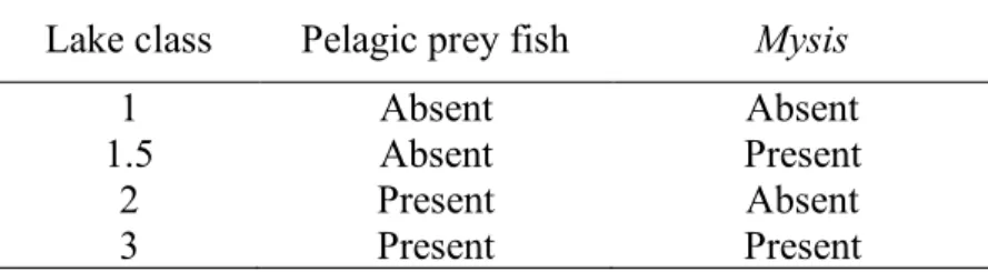
1990). Intermediate trophic levels provide additional links in the food chain; longer food chains potentially result in increased bioaccumulation of metals or contaminants, such as mercury (Oliver and Niimi 1988; Evans et al. 1991). While not present in previous work, I will add a lake category for lakes with Mysis present and pelagic fish absent which will be referred to as Class 1.5 (Table 1). This new class is an extension of food chain length and can potentially aid in explanation of contaminant bioaccumulation.
Table 1. Classification of lake class schemes as described as Rasmussen et al. (1990) with the addition of Class 1.5.
Lake class Pelagic prey fish Mysis
1 Absent Absent
1.5 Absent Present
2 Present Absent
3 Present Present
Mercury toxicity is a major threat to people and wildlife, with methylmercury being the most biologically available and severe form (Celo et al. 2006). In Ontario, mercury pollution is responsible for 85% of prohibitions on human fish consumption from inland lakes (MOECC 2022). Mercury toxicity and poisoning are made more challenging by the bioaccumulation and biomagnification of mercury in food webs.
Apex predators like lake trout have the largest concentrations in their body tissues, in part because they frequently eat food that contains a lot of mercury, and they live longer than forage fishes (Kamman et al. 2005; Swanson and Kidd 2010). Many processes operating at various scales, ranging from the individual fish to the local climate, contribute to the bioaccumulation of fish mercury (Eagles-Smith et al. 2016). Mercury concentrations in freshwater fish are influenced by physiochemical elements connected to lake morphometry and water chemistry (Wren et al. 1991). However, lake trout mercury concentrations are highly variable; this research will address the role of prey assemblages and environmental variables in mercury accumulation in lake trout.
HYPOTHESIS
I hypothesized that changes in food chain length will account for differences in lake trout mercury levels. I predicted that lake trout mercury concentrations would be lowest where no Mysis or pelagic forage fish were found (Class 1) and highest levels where both are present (Class 3). Larger fish will tend to accumulate more mercury due to prey body size and bioaccumulation. As several aspects of lake chemistry have been linked to higher levels of accumulation in the past, I expect that these additional environmental variables will contribute to variation in the concentration of mercury.
LITERATURE REVIEW NATURAL HISTORY OF LAKE TROUT
Lake trout (Salvelinus namaycush), a species in the Salmonidae family, have specific habitat requirements and dietary preferences common to cold-water fishes. Lake trout are native to the northern parts of North America, principally Canada, but also Alaska and, to some extent, the northeastern United States, and they have been
introduced elsewhere (Martin and Olver 1980; Page and Burr 1991). The range of lake trout is most closely associated with the limits of the Pleistocene glacier in North America (Lindsey 1964). Lake trout followed the massive, cold waters that glaciers left behind, which is where they can be found today. In the southern portions of its
distribution in Canada, lake trout are primarily found in deep lakes (i.e., with maximum depths greater than 12.2 m), while in the northern half, particularly in the Territories, they can be found in shallow lakes and rivers (Scott and Crossman 1973).
Lake trout grow slowly and mature late, on average between 6-7 years old but maturity can be as old as 13 years old (Tibbits 2007; Scott and Crossman 1973). They are typically elongate in shape, with total asymptotic length ranging from 381-508 mm.
Lake trout mass can exceed 25 kg in many Canadian lakes but in most inland lakes the average size caught by anglers is less than 4.5 kg (Scott and Crossman 1973). Lake trout like cold, oxygenated water, typically between > 4 – 7 mg·L–1. which greatly reduces the quantity and or quality of habitat that is accessible when lakes are thermally stratified (Blanchfield et al. 2009; Plumb and Blanchfield 2009). Compared to
piscivorous populations, lake trout populations that are mostly planktivorous throughout
the summer have slower growth, smaller body sizes, and inferior growth efficiency (Martin 1966; Pazzia et al. 2002).
Dietary preferences of lake trout vary based on their age and on what prey are available. As a result of the limited postglacial spread of prey taxa and lake
characteristics (such as depth), the length of the food chains leading to lake trout is widely varied, causing their dietary preferences to vary as well (Rasmussen et al. 1990;
Dadswell 1974). Younger lake trout feed primarily on small invertebrates, while adults consume larger prey, like other fishes (Gunn and Pitblado 2004). Zooplankton are present and available to lake trout in all lakes where they are found. However, many lake trout lakes lack preferred intermediate trophic-level prey items, including prey species known as "pelagic forage fish" (smelt, cisco, and whitefish) and Mysis (Vander Zanden and Rasmussen 1996). Although none of these species, especially whitefish, is strictly pelagic, I will continue to refer to them as "pelagic forage fish" to maintain continuity with earlier research.
ENVIRONMENTAL DETERMINANTS OF LAKE TROUT HABITAT OCCUPANCY
Oxy-thermal structure is the main determinant of lake trout habitat occupancy, which changes predictably across seasons. Water temperature and dissolved oxygen concentration (DO) are thought to be the main factors influencing habitat selection by lake trout (Gibson and Fry 1954; Gunn and Pitblado 2004). From early observations, it was noted that lake trout preferred a narrow range of temperatures between 8-12 °C (Ferguson 1958; Coutant 1977; Olson et al. 1988; Christie and Regier 1988). More
recent observations have indicated a broader and colder thermal preference of 5-15°C (Sellers et al. 1998) or < 8°C (Bergstedt et al. 2003). DO thresholds of > 4 mg·L–1 or 6-7 mg·L–1 are commonly used to characterize lake trout habitat requirements (Martin and Olver 1980; Evans 2007; Plumb and Blanchfield 2009). Although these two parameters are rarely measured in situ, management organizations frequently use them to establish standards for the preservation of fish and fish habitat, which explains a large portion of the difference between temperature and DO ranges (Martin and Olver 1980).
Lake trout are considered stenotherms, indicating that their body temperature closely mirrors their surroundings. To achieve optimal physiological function, lake trout must stay within the narrow temperature ranges appropriate to the species (Magnuson et al. 1979; Portner and Knust 2007). Lakes thermally stratify when water in a lake forms distinct layers through heating from the sun and wind. Lakes with cold water generally experience thermal stratification in north-temperate regions throughout the summer, a time when lake trout inhabit the metalimnion (Sellers et al. 1998). In stratified lakes, oxygen deficits in portions of the epilimnion and hypolimnion render the lake unsuitable to lake trout during periods of thermal stratification. Although thermal stratification restricts habitat for cold-water fishes during this time, it is an essential characteristic of north-temperate lakes that keeps the right oxy-thermal habitat available in the summer (Gibson and Fry 1954; Christie and Regier 1988). Lakes would not be able to maintain cold-water species if they mixed completely in the summer since the water would exceed their preferred temperature of >15°C and significantly raises the metabolic costs of occupying warmer and typically littoral habitats.
BIOLOGICAL DETERMINANTS OF LAKE TROUT HABITAT OCCUPANCY AND IMPORTANCE OF FOOD WEB COMPLEXITY
Ecological research has shown that food webs contain a multitude of species-to- species interactions, connecting via multiple links of varying strength species in the same and in different habitats (Vander Zanden and Rasmussen 1996). Food webs are crucial to our comprehension of the stability and function of ecosystems. Complexity, also known as connectance, is a crucial component of food web structure; it is the number of food web links expressed as a proportion of all possible links (Beckerman et al. 2006).
Many factors affect the structure of food webs and the life history traits of fish (Pazzia et al. 2002). According to fish growth models, foraging expenses rise when a predator's size increases in relation to its prey because it needs to find and eat more prey to meet its energy needs (i.e., decreased growth efficiency; Kerr 1971; Giacomini et al.
2013). Fish feeding on smaller prey are predicted to have higher foraging expenses as their body size increases stratification. Lake trout typically inhabit oligotrophic lakes, characterized by low nutrients and productivity. Salmonids in that live northern lakes have a short growing season and in response typically grow slower and live longer lives (Johnson 1972). The capacity of a lake trout to choose habitat can also be influenced by harvest pressure, since harvest causes behavioural changes such as individual boldness or shyness (Uusi-Heikkila et al. 2008). Behavioural changes can cause fish to be less effective foragers, have reduced mating success, and possibly also have lower parental caregiving abilities.
Cold-water predators exhibit seasonality in their foraging in response to
stratification, relying on pelagic energy sources like zooplankton and macroinvertebrates (such as Mysis or Chaoborus) when surface and littoral waters are too warm in the summer. Lake trout tend to feed in the littoral zone when they are cooler in the spring and fall (Martin 1952; Guzzo et al. 2017). When thermal stratification occurs, portions of the epilimnion and hypolimnion become unavailable, making the thermocline a preferable foraging habitat. In the summer, lake trout reduce their use of littoral habitat and occupy deep pelagic waters (Guzzo et al. 2017). Lake trout and many other
predatory fish in north-temperate lakes are guided in their foraging behaviour by fluctuations in prey density and seasonality. Lake trout populations must have suitable prey species present throughout the year in their thermal range for rapid growth (Scott and Crossman 1973; Pazzia et al. 2002). Lack of adequate prey can prevent fish from switching to larger prey, affecting the content, and structure of the food web (Martin 1952).
In both littoral and pelagic environments, freshwater fish encounter prey populations with uneven size spectra, little to no biomass, and mismatched abundance, all of which can affect population growth rates (Werner and Gilliam 1984). Typically, oligotrophic lakes consist of few species of zooplankton, invertebrates, and intermediate species such as Mysis or forage fish (Ryder and Johnson 1972). When Mysis are present, they can play a significant role in the diet of young lake trout, but diet of larger
individuals diets are often dominated by minnows (Cyprinidae), cisco (Coregonus artedi), slimy sculpin (Cottus cognatus), and yellow perch (Perca flavescens) when they
are available. Mysis can also serve as a major food source for older lake trout if they are highly abundant (Konkle and Sprules 1986; Trippel and Beamish 1993).
THE CONCEPT OF LAKE CLASSES
To directly assess how the presence and/or absence of key prey items affects predator traits (such as mercury accumulation), a categorical grouping of prey availability to lake classes can be useful. The idea of lake classes is based on trophic levels, whereby species are grouped into trophic level groupings and then handled as distinct categories in subsequent modeling (Vander Zanden and Rasmussen 1996). An effective example of lake classes being used to describe population-level differences across a gradient of food web complexity was in the work of Rasmussen et al. (1990).
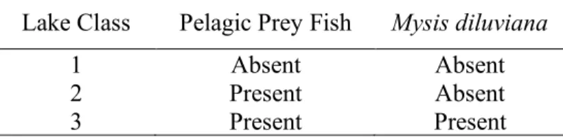
Rasmussen described lake classes by dividing lake trout lakes into groups based on the presence or absence of simple intermediate prey species (Table 2). Rasmussen’s study assessed how food chain length explains differences in polychlorinated biphenyls (PCBs), which are contaminants within aquatic ecosystems (Rasmussen et al. 1990).
The study found that PCB levels in lake trout increase with the length of the pelagic food chain; trout from the shortest food chains (Class 1 lakes) had the lowest PCB levels, and those from the longest food chains (Class 3) had the highest levels. The results provided evidence of food chain biomagnification, although the authors did not comprehensively assess all combinations of lake class types in their study.
Table 2. Classification of lake class schemes as described as Rasmussen et al. (1990).
Lake Class Pelagic Prey Fish Mysis diluviana
1 Absent Absent
2 Present Absent
3 Present Present
MERCURY CONCENTRATION IN AQUATIC SPECIES
Mercury is categorized as a neurotoxin that poisons both humans and wildlife by penetrating organisms through the absorption of different forms of mercury (Celo et al.
2006). The symptoms of mercury poisoning in people can range from neurological impairments, respiratory problems, fertility issues, cardiovascular problems, immune system compromise, and fetal abnormalities, to death (Ullrich et al. 2001; Lourie 2003;
Gonzalez-Raymat et al. 2017). The aquatic ecosystem is a main source of mercury exposure for humans and wildlife since methylmercury is stored in fish muscle tissue (MOECC 2022).
Elemental mercury (Hg0) can be introduced into the environment by both natural sources and anthropogenic activities. Natural sources include volcanoes, forest fires, oceanic emissions, and the natural degassing of the earth's crust. Present-day
anthropogenic sources of global mercury (Hg) have been studied for more than a decade (Streets and Zhang 2009). Abiotic or biotic processes have the ability to methylate elemental mercury, which can then change inorganic mercury into the hazardous form of methylmercury that is carried by water bodies (Celo et al. 2006). Methylmercury is the most prevalent and severe form of mercury toxicity. The numerous complex interactions within the mercury cycle involve methylation, demethylation, and biotic
processes. Methylmercury bioaccumulates in aquatic ecosystems by binding to tissues within organisms (Ullrich et al. 2001).
Bioaccumulation occurs when contaminants are taken up by the organism faster than they can be eliminated (Lourie 2003). Further, biomagnification is when
increasingly larger amounts of mercury accumulate with increasing trophic levels. As a result, top predators, like lake trout, have high levels of methylmercury in their body tissue because of biomagnification increasing with food chain length, and individual bioaccumulation because of slow growth rates and contaminated prey (Kamman et al.
2005).
Mercury is a dangerous global contaminant due to its widespread distribution and deposition into terrestrial and aquatic systems (Fitzgerald et al. 1998). Several variables affect the amount of mercury that accumulates in freshwater fishes, including fish size, waterbody pH, dissolved organic carbon, watershed features, algal
productivity, and zooplankton community structure (Driscoll et al. 1994; Kamman et al.
2003; Chen et al. 2005). In response to bioaccumulation and biomagnification, mercury concentrations in fish tend to increase with fish age, size, and trophic position. While older larger fish tend to have higher mercury, mercury will usually, but not always, decrease with faster growth and greater body condition (Evans et al. 2005). The
concentration of contamination rises with each level of a food chain as its consumed by the producer and gradually transferred to the top of that food chain (Fitzgerald et al.
1998).
Due to the high toxicity of mercury, Health Canada has set a guideline for the maximum average level of mercury in fish for commercial sale at 0.5 parts per million
(ppm) for human consumption (MOECC 2022). In addition, guidelines have been set on consuming herring, salmon, smelt, trout, and lake whitefish, with a suggested limit for consumption is approximately 150 grams per week for the general population while children are recommended to eat even less (MOECC 2022). Previous studies have found that whole-body values of 10–20 μg/g can be lethal to most fish (Niimi and Kissoon 1994). Fish and potentially other aquatic organisms may be affected chronically by whole body mercury concentrations of 1- 5 μg/g. Low levels of mercury pollution can indirectly impact fish populations by disrupting physiological processes as opposed to neurological impairment and death that can be brought on by high contamination levels (Crump and Trudeau 2009). Previous studies on Atlantic salmon and Rainbow trout showed that mercury exposure of 10 μg/L of methylmercury or muscle content of above 0.6 μg/g has been linked to brain lesions, oxidative stress, decreased activity, and/or rendered inactive gonadotrophic hormones, which are released from the pituitary in fish.
Mercury contamination can also affect reproductive function; previous studies have found a threshold of 0.2 μg/g, and concentrations exceeding the limit affect the control of the annual cycle of gonadal growth, ovulation in females, sperm release in males, and production of sex steroids in both sexes that cause impotence (Crump and Trudeau 2009; Berntssen et al. 2003; Breton et al. 1998). These biological implications occur after long-term dietary exposure to mercury.
ENVIRONMENTAL VARIABLES
Lake characteristics and water chemistry are two factors that can influence mercury methylation and demethylation processes (Garcia and Carignan 2000). Fish
mercury accumulation is influenced by a number of environmental and biological factors, such as pH and trophic position (Cabana et al. 1994). Based on their importance in previous literature, this study focused on four main variables: dissolved organic carbon (DOC), pH, total dissolved phosphorus (TDP), and lake morphology.
At the landscape and biogeochemical levels, there are substantial connections between the cycles of mercury and carbon. Dissolved organic carbon (DOC) may bind to a variety of trace metals, including mercury (Mason 2013). Many studies have revealed a strong linear association between DOC concentrations in water and total mercury (THg) or methylmercury (MeHg) concentrations in freshwater environments (Grigal 2002; Riscassi and Scanlon 2011; Stoken et al. 2016). These studies and others suggest that DOC may have a mitigating effect on the production and/or
bioaccumulation of MeHg in water. Many of the mechanisms for the mobilization and transformation of mercury (Hg) and DOC to freshwater ecosystems have been identified (Lavoie et al. 2019). In freshwater ecosystems, mercury is carried from the catchment basin and has the potential to be methylated while travelling through marshes, streams, rivers, and lakes, where there is a strong but variable coupling between carbon and mercury cycles. This coupling is influenced by regional factors like geography, time, and human activity, and has implications for understanding biogeochemical processes that are also rapidly changing in response to climate change (Lavoie et al. 2019).
Previous studies have been conducted to determine if pH will directly alter the bioaccumulation of MeHg in fish, but the findings are inconsistent. Nonetheless, the bulk of studies revealed that lakes with low pH typically have fish with higher mercury concentrations (McMurtry et al. 1989; Greib et al. 1990; Suns and Hitchin 1990; Wiener
et al.1990). Concern over the ecological effects of acid deposition has heightened interest in the function of pH and alkalinity in mercury accumulation. Fish in lakes with lower pH values typically have greater amounts of methylmercury, which increases the bioavailability of mercury (Garcia and Carignan 2000; Weiner et al 2006).
It has long been believed that phosphorus, an essential nutrient for the
development of aquatic plants and algae, is a major factor in the overall productivity of freshwater ecosystems (Gov. of Can. 2015). An increase in phosphorus can expedite fish growth and reduce fish mercury through growth dilution (Rypel 2010). According to one study, aquatic ecosystems are more vulnerable to mercury contamination in fish when fish have reduced growth rates, which are linked to low growth efficiency. With an increased metabolism, fish tend to consume food at faster rates that can increase mercury accumulation (Ward et al. 2010). A multi-lake study from northeastern North America found a link between higher mercury bioaccumulation in food webs and relatively low lake productivity (Chen et al. 2005). A Canadian lake study (Kidd et al.
2012) discovered a positive relationship between phosphorus levels and
biomagnification of total mercury in food webs, and fish communities. The amount of methylmercury in fish can also be decreased by increasing lake primary productivity, which can occur when mercury levels in lake food webs are diluted (Pickhardt et al.
2002).
The ratio between methylation and demethylation rates is strongly temperature dependent (Bodaly et al. 1993). Temperature-dependent increases in biological activity and chemical reaction rates lead to an increase in the rate of mercury methylation
(Bigham et al. 2016). According to Ullrich et al. (2001), the rate of mercury methylation
often peaks in aquatic systems during summer, demonstrating the significant impact of temperature on overall Hg methylation. Temperature in turn is related to lake surface area and surface depth; small lakes are generally shallower, and typically respond more quickly to atmospheric temperature, making them warmer in the summer and colder in the winter. More total mercury accumulation in lake trout tissues is caused by higher water temperatures, which favour methylmercury transformations over demethylation (Bodaly et al. 1993).
METHODS AND MATERIALS STUDY AREA
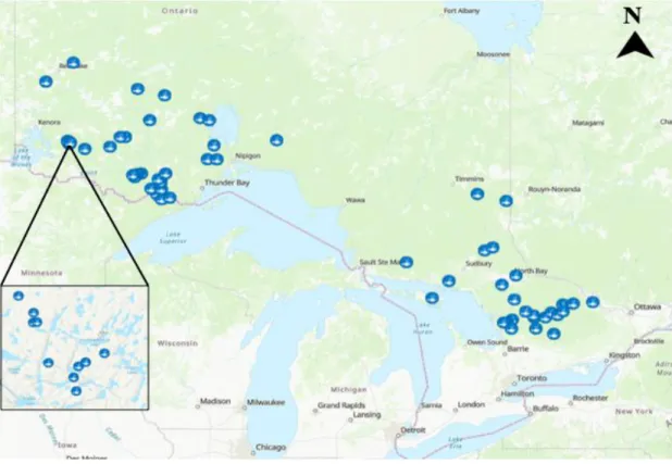
Fish and water samples were collected from the Ontario’s Broadscale Monitoring (BsM) Program and from the long-term dataset collected at the IISD- Experimental Lakes Area (ELA) located in Northwestern Ontario (Figure 1). The BsM Program collaborated with the Ontario Ministry of Natural Resources and Forestry and the Ministry of the Environment and Climate Change to analyze samples and
subsequently develop databases of mercury contaminant concentrations in fish across Ontario (OMNR 2009). A number of lakes were also selected from the IISD-ELA to provide additional samples to ensure adequate numbers of samples for each lake class (Class 1, 1.5, and 3). A total of 64 lakes were selected to obtain data from mercury analysis and on environmental variables from (Table 3).
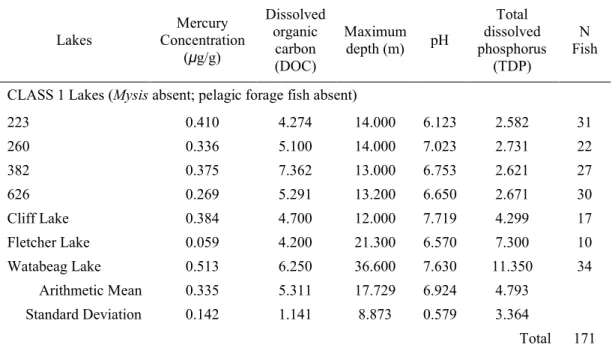
Table 3. Average mercury concentration of lake trout from Ontario lakes with different pelagic communities with the average environmental measurements from each lake and total fish sampled.
Lakes Mercury
Concentration (μg/g)
Dissolved organic
carbon (DOC)
Maximum depth (m) pH
Total dissolved phosphorus
(TDP)
Fish N
CLASS 1 Lakes (Mysis absent; pelagic forage fish absent)
223 0.410 4.274 14.000 6.123 2.582 31
260 0.336 5.100 14.000 7.023 2.731 22
382 0.375 7.362 13.000 6.753 2.621 27
626 0.269 5.291 13.200 6.650 2.671 30
Cliff Lake 0.384 4.700 12.000 7.719 4.299 17
Fletcher Lake 0.059 4.200 21.300 6.570 7.300 10
Watabeag Lake 0.513 6.250 36.600 7.630 11.350 34
Arithmetic Mean 0.335 5.311 17.729 6.924 4.793
Standard Deviation 0.142 1.141 8.873 0.579 3.364
Total 171
Lakes Mercury Concentration
(μg/g)
Dissolved organic
carbon (DOC)
Maximum depth (m) pH
Total dissolved phosphorus
(TDP)
Fish N
CLASS 1.5 Lakes (Mysis present; pelagic forage fish absent)
224 0.293 3.118 27.000 6.845 2.852 144
373 0.338 3.974 21.000 7.031 4.163 59
375 0.336 6.220 27.000 7.309 3.981 65
442 0.333 6.395 18.000 6.891 2.937 24
Burchell Lake 0.516 4.900 74.700 7.275 3.100 41
Cry Lake 0.292 2.400 47.600 7.200 13.100 43
Grouse Lake 0.341 4.299 38.400 7.339 8.900 14
North Lake 0.186 3.300 36.000 7.380 13.600 20
Squeers Lake 0.192 3.899 33.600 7.290 9.300 26
Twinhouse Lake 0.595 7.500 15.000 6.610 5.700 18
Walotka Lake 0.462 6.050 23.000 7.095 4.300 45
Arithmetic Mean 0.353 4.732 32.845 7.115 6.539
Standard Deviation 0.126 1.611 16.898 0.246 4.030
Total 499
CLASS 2 Lakes (Mysis absent; pelagic forage fish present)
Aylen Lake 0.819 3.450 67.100 7.000 3.850 48
Bark Lake 0.500 4.800 87.500 6.545 7.050 24
Bella Lake 0.234 2.700 36.600 6.800 7.200 31
Bending Lake 0.797 8.000 45.800 6.790 5.900 10
Cobre Lake 0.100 2.300 61.600 7.300 1.700 2
Eels Lake 1.020 4.800 29.900 7.100 7.300 22
Emerald Lake 0.178 2.250 48.800 7.000 3.400 50
Kawagama Lake 0.379 3.200 77.000 6.580 3.600 74
McKenzie Lake 1.662 5.750 27.400 6.685 6.250 18
Opeongo Lake 0.560 4.800 51.100 7.050 4.800 47
Smoke Lake 0.274 3.700 56.100 6.810 3.300 35
Arithmetic Mean 0.593 4.159 53.536 6.878 4.941
Standard Deviation 0.460 1.714 18.912 0.233 1.906
Total 361
CLASS 3 Lakes (Mysis present; pelagic forage fish present)
239 0.713 6.489 30.000 6.905 3.100 21
468 0.400 NA 29.000 NA NA 49
Arrow Lake 0.394 2.950 54.900 7.289 5.050 90
Bear Lake 0.242 2.799 54.000 7.049 7.299 20
Black Sturgeon Lake 1.425 11.050 52.400 7.570 6.350 28
Lakes Mercury Concentration
(μg/g)
Dissolved organic
carbon (DOC)
Maximum depth (m) pH
Total dissolved phosphorus
(TDP)
Fish N
Carling Lake 0.582 12.350 40.900 7.190 11.600 18
Clear (Watt) Lake 0.253 4.400 40.000 6.920 7.000 36
Crystal Lake 0.283 2.600 47.000 6.950 4.900 60
Eva Lake 0.497 7.300 54.900 7.269 12.650 50
Indian Lake 0.782 5.300 36.000 7.230 8.950 5
Kashabowie Lake 0.710 10.550 35.000 6.920 8.650 2
Lake Bernard 0.341 3.366 47.900 7.033 10.866 16
Lake Joseph 0.322 2.962 92.000 6.886 5.650 138
Lake Manitou 0.193 4.299 49.100 8.009 5.200 184
Lake Muskoka 0.677 4.300 66.500 6.700 7.500 86
Lake Rosseau 0.569 3.799 89.000 6.870 5.516 116
Lake Temagami 0.332 2.950 75.900 6.980 4.800 68
Larder Lake 0.345 5.700 33.500 7.635 8.300 67
Long Lake 1.398 9.750 186.100 7.925 10.650 74
Longlegged Lake 1.037 8.850 35.400 7.175 19.600 28
Lower Manitou Lake 0.440 5.300 81.000 7.265 5.950 25
Mameigwess Lake 0.532 2.900 50.000 7.420 5.250 65
Muskrat Lake 0.429 6.900 64.000 8.195 39.600 42
Northern Light Lake 0.197 9.900 39.700 7.030 10.550 14
Nym Lake 0.728 5.100 37.200 6.870 6.600 6
Obonga Lake 2.900 8.850 71.700 6.950 6.050 2
Pickerel Lake 0.637 6.600 74.700 6.950 6.750 80
Round Lake 0.762 5.750 54.900 7.185 7.650 70
Savant Lake 0.815 7.550 53.000 7.155 6.000 10
Skeleton Lake 0.367 1.700 61.000 7.000 2.700 76
Sturgeon Lake 0.823 6.050 93.000 7.385 6.500 15
Titmarsh Lake 0.789 6.149 49.400 6.990 5.700 76
Trout Lake 0.918 4.500 47.300 7.435 5.500 39
Trout Lake 0.349 3.100 69.200 7.144 5.100 86
Twelve Mile Lake 0.308 3.300 27.500 7.005 5.349 74
Arithmetic Mean 0.643 5.747 57.803 7.191 8.202
Standard Deviation 0.497 2.770 28.712 0.344 6.388
Total 1836
With a total of 2,867 samples, 2,770 samples were previously analyzed with results provided and the additional 97 samples were analyzed during the duration of this thesis to provide supplementary results for the variety of lake classes (see Appendix I and II). Mercury samples from ELA were collected between 1972 and 2022, and samples from BsM between 1993 and 2019.
Figure 1. Lakes sampled in Ontario’s Broadscale Monitoring Program and IISD- Experimental Lakes Area for this study.
FISH COLLECTION AND SAMPLING
Broadscale Monitoring Program (BsM) Sampling Protocol
In order to track the condition of Ontario's inland lakes, the Ontario Ministry of Natural Resources (OMNR) developed the Broad-scale Monitoring (BsM) program in 2008 (OMNR 2009). To reduce sample bias, a random stratified data collection was used. Beginning in late May, when the water surface temperature reaches 18 °C or
above, netting is carried out (Sandstorm et al. 2013). Field collection ends when surface temperatures falls below 18 °C.
A large mesh gillnet (known as a North American, NA1) is a standard for sampling angler harvested freshwater species in North America, with eight different mesh sizes per gang (stretch measurements: 38, 51, 64, 76, 89, 102, 114, and 127 mm) is used to catch fish (Sandstorm et al. 2011). Every depth stratum and area of the lake received equal consideration. The nets are normally set between 13:00 and 17:00 hours and left overnight before being taken down between 08:00 and 11:00 hours the next day.
The minimum and maximum immersion times for large nets and small nets, respectively, are sixteen and twenty-two hours, and twelve and twenty-two hours, respectively (Sandstorm et al. 2013). Each fish's measurements, including length, weight, age estimation (from scales and otoliths) and sample site, are noted. A tissue sample from the dorsal muscle tissue is collected to analyze for heavy metals including mercury. A sample size of no less than 100 grams is necessary. Guidelines on the recommended eating portions and frequency of fish consumption are created using the information gathered.
Experimental Lakes Area (ELA) Sampling Program
The fish program at IISD- Experimental Lakes Area monitor the health of fish species by sampling fish using various methods. In order to determine population
abundance and structure in many of the lakes, IISD-ELA staff employ mark-recapture in the spring and fall. Trap nets are used during spring and in the fall, when 38 mm short- set gillnets (10–20 min) are added to trap net samples to catch lake trout on spawning
shoals just after dusk. Fish were caught in all lakes using a minimum of two Beamish- style trap nets during the spring and autumn sample periods (Rennie et al. 2019). There are two different kinds of trap nets: those with a central lead that is positioned
perpendicular to the shore (Beamish 1972), and those without a central lead that have one wing tied to the shore and positioned roughly parallel to the shoreline in order to catch fish moving in a single direction. The mesh size of trap nets used is approximately 3 mm, with a weekly cycle of 4-6 weeks, emptied every 2-5 days depending on the water temperature. The number and size of each fish caught in the nets is recorded (Rennie et al. 2019). Captured fish are measured for length, weight, and age estimation (from a fin ray clip), and tissue samples are taken from the dorsal muscle to use for laboratory testing.
ENVIRONMENTAL SAMPLES
Environmental variables were taken from each lake in this study, including dissolved oxygen, temperature, water chemistry, and lake morphology (surface area, minimum and maximum depth). Water samples from the BsM lakes were sent to the Ministry of the Environment and Climate Change for chemical analyses to determine pH, total dissolved phosphorus (TDP), and dissolved organic carbon (DOC).
MERCURY ANALYSIS
A total of 2,867 samples were evaluated; 2,770 samples had findings from prior analysis; the remaining 97 samples were analyzed over the course of this thesis to offer additional data for the various lake classes (see Appendix I and II). The 97 samples were
from 1984 to 2022, all of which were collected from IISD-ELA. These samples were analyzed using Milestone’s Direct Mercury Analyzer (DMA 80). The DMA was
calibrated, primed, and operated following the EPA method 7473 (Peterson et al. 2015).
The samples were quality controlled by including sample blanks and standard reference materials. Every five samples were subjected to a duplicate run for quality control, two blanks, and a standard reference material (SRM). TORT-3 (lobster
hepatopancreas and fish protein) was used as the SRM to evaluate ongoing precision of the DMA. In each sample run (which contained up to 20 mercury samples) completed, the standard's mean estimations ranged between 0.27 - 0.29 mg/kg, which is within the SRM's 0.292 0.022 mg/kg permitted ranges. To assess lake trout mercury
concentrations, a small piece of muscle tissue was removed from the dorsal muscle with a scalpel in order to prepare the sample for examination. Using a microbalance on a metal weigh boat, the sample was weighed, and the results were entered into the DMA program. The cut sample typically weighed 0.06 to 0.09 g. The machine's slots were filled with each weigh boat containing the weighted sample. The analyzer ran until it was finished, usually taking six hours. The results were then saved to an Excel file. Any sample that fell outside of the acceptable range because of the muscle's abnormally high or low mercury concentration was rerun to assure reliable results. Blanks on the DMA were accepted if they were less than 0.003 mg/kg mercury concentration.
STATISTICAL ANALYSIS
All analyses were conducted using R (version 3.6.2., 2023 R core team). An Analysis of Covariance (ANCOVA) was attempted to analyze the relationship between
mercury concentrations with body size between lake classes, but due to a statistically significant interaction term (i.e., the slope of the relationship between lake class and mercury was not consistent across body size), the ANCOVA was deemed unfit. Instead, a Linear Mixed Effect Model (LMM) was used with lake class as a fixed factor and lake trout body size as a covariate, a random slope for body size and a random intercept of lake class. An LMM allows easing of the assumption of independent observations (repeatedly sampling fish from a single lake) by accounting for that non-independence.
The optimal model was chosen using stepwise deletion of random and fixed effects. To assess model fit, likelihood ratio tests were used, and it was determined that the best LMM had lake class and body size as fixed factors and a random slope and intercept for lake trout body size and lake class, respectively.
A principal component analysis (PCA) was used to assess the association between environmental variables, lake morphology, lake class, and mercury
concentrations. Five variables were selected; dissolved organic carbon (DOC), pH, total dissolved phosphorus (TDP), and lake morphology (surface areas and maximum depth).
Only maximum lake depth was retained for lake morphology variables as an initial scatterplot of all variables showed that lake area (ha) and maximum depth (m) were highly correlated. Environmental factors that were to be analyzed were chosen after they were assessed and plotted to ensure they are “normally” distributed then the data was standardized. A biplot of the PCA was then created to describe associations between all variables.
RESULTS
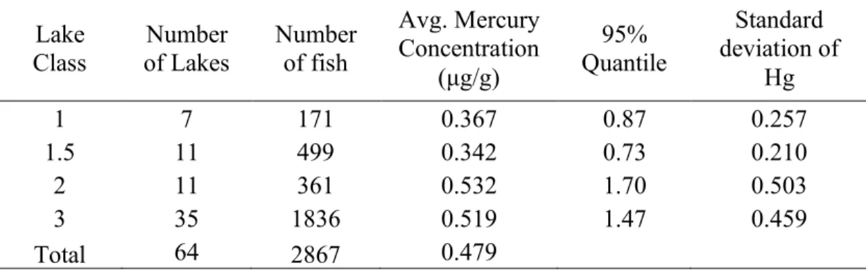
There was a total of 64 lakes sampled and 2,867 samples analyzed across the lake classes. The average mercury concentration for lake trout increased with increasing lake class, but the standard deviation of mercury concentrations also increased as well (Table 4).
Table 4. Summary of lake class values (number of lakes and individual samples
analyzed) and average mercury concentration with 95% quantile and standard deviation values.
Lake
Class Number
of Lakes Number of fish
Avg. Mercury Concentration
(μg/g)
Quantile 95%
Standard deviation of
Hg
1 7 171 0.367 0.87 0.257
1.5 11 499 0.342 0.73 0.210
2 11 361 0.532 1.70 0.503
3 35 1836 0.519 1.47 0.459
Total 64 2867 0.479
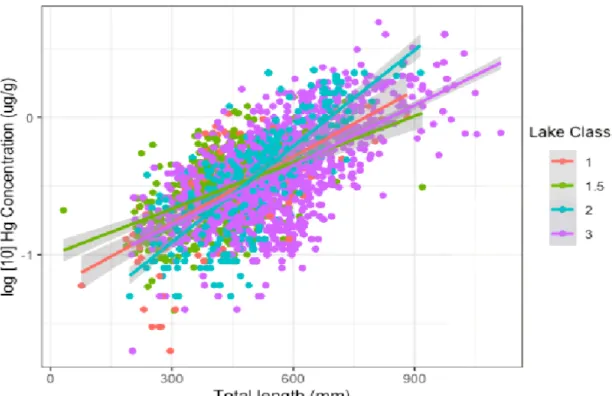
There was a significant effect of lake class (LMM, F3,116.49 = 3.12, p = 0.029) and body length (LMM, F1,113.45 = 558.36, p < 0.0001) on lake trout mercury concentrations.
However, a significant interaction between body length and lake class (LMM, F3,104.04 = 5.92, p = 0.0009) suggests that increases in mercury concentrations with body size are not consistent across lake classes; mercury increased with body size fastest in Class 2 lakes, and slowest in Class 1.5 lakes (Figure 2). Slopes from the LMM suggest that a 500-mm fish is likely to have a mercury concentration of approximately 0.35 μg/g regardless of what lake class they are in, but that fish larger than 750 mm in Class 2 lakes will have higher mercury concentrations than fish from other lake classes.
Figure 2. Comparison of log-transformed Hg concentration with total length across lake classes (R2 = 0.481).
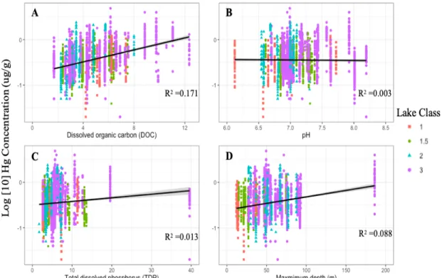
In this study, environmental variables were found to have relationships with lake trout mercury concentration. Dissolved organic carbon (DOC) had the highest
significantly positive relationship with an R2 value of 0.171 which explains 17.1%
variation within the data (linear regression, F1,2816 = 581.8, p < 0.001), while pH had the least positive relationship, meaning a p value closest to 0.05 and only explaining 0.3%
(linear regression, F1,2816 = 8.22, p = 0.004). Maximum depth explained 8.8% variation (linear regression, F1,2816 = 272, p < 0.001), and total dissolved phosphorus (TDP) explained 1.3% (linear regression, F1,2816 = 37.08, p < 0.001) with p values lower than 0.05 indicating there is a significant relationship between those variables and mercury concentrations but R2 values indicating that the relationship explains very little (Figure 3).
Figure 3. Comparison of the influence of environmental variables on mercury
concentration across lake classes. A. Dissolved organic carbon (DOC) B. pH C. Total dissolve phosphorus D. Maximum depth (m).
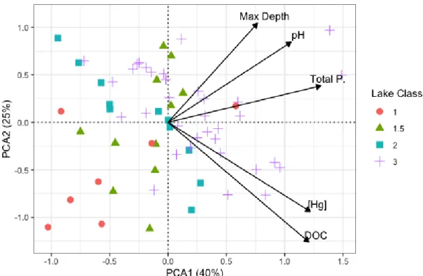
A PCA plot was graphed to assess the association between lake classes environmental variables on mercury concentrations (Figure 4). The first two PC axes explained 65% of total variation. The first axis (PC1) shows a general association between all variables, showing that lakes with higher Hg have more complex food webs, are deeper, and higher in DOC, phosphorus and pH. The second axis (PC2)
demonstrates that high DOC lakes have higher mercury concentrations. Figure 4 demonstrates there are two distinct groups, one corresponding to high DOC and higher Hg concentration, and the other group corresponding to deeper, higher pH and higher total phosphorus. Both groups tend to correspond to Class 3 lakes.
Figure 4. Principal component analysis (PCA) biplot of environmental variables and mercury concentration across lake classes.
DISCUSSION
My results demonstrated a significant effect of body length and lake class on lake trout mercury concentration, but that increases in mercury concentrations with body size are not consistent across lake classes. This effect contradicts my original prediction that mercury concentrations would increase when aquatic food chains lengthen. When evaluating mean mercury concentrations for each lake class in a way similar to that of Rasmussen et al. (1990), my results show mercury concentrations closer to my
predictions (Table 4; with the exception that Class 2 is slightly more elevated than Class 3). However, when body size is accounted for, these predictions were not supported.
Further analysis of environmental variables demonstrates that assessing other environmental variables (DOC, pH, TDP, and maximum depth) can be useful when describing lake trout mercury concentrations across a large landscape.
According to early research on ecosystem behaviour of organic pollutants, such as that by Rasmussen et al. (1990) and Oliver and Niimi (1988) examining PCB levels, this study contradicts previous findings of contaminant biomagnification when aquatic food chains lengthen. Some differences between the Rasmussen et al. (1990) study are important to note. Previous studies assessed lake averages for all sampled fish rather than using body-size as a covariate within a lake. Contaminant levels tend to increase with fish size, and by using body size as a predictor aids in accounting for the size variation within a lake class. Additionally, samples from Rasmussen et al. (1990) were taken between 1978 and 1981, whereas those used in this study were taken between 1972 and 2022, with the majority coming from the last decade or two. Between 1990 and 2010, atmospheric mercury emissions declined by 85% in Canada, with the
reduction truly starting since the 1970s (MOECC 2022). Globally, mercury emissions remained stable between 1990s and 2000s. As of 2020 in Canada, mercury emissions decreased drastically respectively from 1990 levels, mostly due to a large reduction in the non-ferrous refining and smelting industry (ECCC 2022). The large decrease in mercury emissions over this time could be a factor into why this study’s results did not reflect the same relationship seen between accumulation of contaminants and lake classes as Rasmussen et al. (1990) did.
My results indicate that both DOC and maximum lake depth are useful
predictors of lake trout mercury concentrations. Linear regression demonstrated a strong relationship between DOC and mercury (R2 = 0.171; Figure 3 Panel A). Additionally, there was a close association between DOC and lake depth, with PC axis 2, describing DOC and lake depth, accounting for 25.9% of the overall model variation (17.1 and 8.8% respectively; Figure 4). Several studies have supported the positive relationship between DOC and fish mercury (Ullrich et al. 2001, Grigal 2002, Weiner et al. 2006, and Gonzalez-Raymat et al. 2017), and larger and deeper lakes can have lower mercury concentrations due to the lower methylation potential for cooler surface waters (Bodaly et al. 1993). Furthermore, it is likely that the association between DOC and lake depth is a function of water residency time and lake volume. Lakes with low DOC are
commonly connected to relatively big, deep lakes (high water volume) with slow water turnover, whereas lakes with the greatest DOC are typically found in small, shallow (low water volume) lakes with shorter water residency times (Grigal 2002; Rasmussen et al. 1989). While counterintuitive, shorter water residence times may allow for a larger influence from watershed processes. The binding potential of mercury to terrestrial-
derived organic carbon and other trace metals, may lead to higher mercury
concentrations for lakes and fish from shallower and smaller lakes, as was seen across the lakes within this study (Ullrich et al. 2001).
Phosphorus and pH both had a statistically significant relationship with mercury concentrations, yet with a combined R2 of <0.02, they are not useful predictors of lake trout mercury concentrations. This study found that pH alone explained only 0.3% (R2 = 0.003). The poor signal I saw between mercury and pH may be due to the complex, and oftentimes contradictory effects, of mercury concentrations and pH found within the literature. While many studies have suggested a positive relationship between acidified lakes and mercury levels (Greib et al. 1990; Suns and Hitchin 1990; Wiener et al. 1990), others have found that predatory fish did not have high levels of methylmercury and lake water acidity was not a major influence in methylation (Lucotte et al. 2016). The contrasting results require further investigation and consideration needs to be given to any number of possible factors that could impact results. This study only observed pH ranges from 6.123 to 8.195, while studies such as Suns and Hitchin (1990) studied lakes with a smaller pH range of 5.6 to 7.3, potentially explaining the differences in results.
Phosphorus explains little variation but in particular follows the lake class gradient shown in the PCA (Figure 4); food web effects (i.e., lake class differences) may be masking any productivity effects that were anticipated. Similar to pH, there are conflicting reports on the effect of phosphorus on mercury concentrations. Since phosphorus is often related to lake productivity, it can expedite fish growth and reduce fish mercury through growth dilution (Rypel 2010). Other studies find that increased phosphorus may promote cyanobacterial growth, lake eutrophication, and organic
material (such as DOC) for mercury deposition in the watershed, which can lead to increased mercury within fish (Krutzweiser et al. 2008).
Overall, the mean mercury concentration in lake trout across all study lakes was 0.479 μg/g, with Class 2 and Class 3 lakes exceeding average concentrations (0.532 and 0.519 μg/g respectively). Class 2 and Class 3 values exceed what is deemed acceptable for human consumption, as mercury concentrations below 0.5 ppm (or 0.5 μg/g) are recommended under consumption guidelines (MOECC 2022). The total mean mercury concentration is just below the recommended concentration. Eating fish that contains mercury, a neurotoxin, can have serious health effects. By keeping fish consumption below advised limits, toxicity thresholds should not be reached, and symptoms of mercury poisoning should be avoided (MOECC 2022). Encouragingly, a whole
ecosystem study demonstrated that when mercury deposition decreases, methylmercury levels in Northern pike (Esox lucius) soon followed (Blanchfield et al. 2021).
CONCLUSION AND RECOMMENDATIONS
This study provides evidence that landscape and lake chemistry factors, such as pH, total dissolved phosphorus, and maximum lake depth, have an impact on the total mercury levels in top predatory fish. This study, however, does not support the use of lake classes to assess mercury levels, as the results did not confirm previous findings once fish body size was accounted for. Although our findings could not conclude the relationship between lake classes and mercury concentration, by exploring
environmental variables it was concluded that DOC has a strong positive relationship (17.1%) with fish mercury concentration. While environmental variables collectively explained 27.5% of the variation in mercury concentrations, DOC was the most
important environmental variable (R2 = 0.17), with lake maximum depth also explaining a statistically and biologically significant amount of variation in lake trout mercury concentrations (R2 = 0.09). This study finds that the environmental variables explored are the most important factors driving the results seen. To fully comprehend
bioaccumulation and biomagnification and to assess the neurotoxic effects on human and wildlife health, it is crucial to continuously monitor mercury quantities in the environment and the wildlife we eat.
It is advised to conduct more research in order to better comprehend the environmental elements that affect the accumulation, methylation, and mobilization of mercury as well as to examine the precision and prospective applications of lake classes.
It is advised that monitoring efforts be strengthened in order to validate mercury trends and produce data for management actions, such as issuing thorough fish consumption recommendations to safeguard human health. Additional research is required for
analysis and accuracy in order to fully comprehend the mechanisms causing mercury pollution in Ontario's inland lakes. Identifying variation in mercury due to the many factors of ecosystem and watershed variation can allow for more accurately estimated mercury concentrations of fish across large landscapes. We can hope that international efforts to reduce mercury risk, growing understanding of how mercury behaves in the environment, and actions on climate change will lower fish mercury levels.