UNIVERSITAT POLITECNICA DE CATALUNYA
DEPARTAMENT DE TEORIA DEL SENYAL ï COMUNICACIONS
TESI DOCTORAL
HIGHERORDER STATISTICS APPLICATIONS IN
IMAGE SEQUENCE PROCESSING
AUTOR : ELISA SAYROL CLOLS
CHAPTER 4
MOTION ESTIMATION USING HIGHER-ORDER STATISTICS
In this chapter we propose a class of cost functions based on HigherOrder Statistics, to estimate the displacement vector between consecutive image frames. In case the sequence is severely corrupted by additive Gaussian noise of unknown covariance, using higher than second order statistics is appropriate since cumulants of Gaussian noise are zero. To obtain consistent cumulant estimates we need several records of the same sequence, which is not generally possible. Nevertheless, previous frames, where the registration problem has already been solved, can be used to obtain asymptotically unbiased estimates. This is possible when stationarity among the employed frames can be assumed. The objective of this work is to introduce HOSbased cost functions capable of estimating motion even for small regions or blocks. An alternative estimation is also provided, when only two frames are available, that outperforms other higherorder statisticsbased cost functions. Finally, a recursive version to obtain the displacement is derived for cases when some a priori knowledge is available.
4.1 Introduction
An image or video sequence is a series of 2D images sequentially ordered in time. There is a growing interest in research applications involving image sequences, mainly in the area of image sequence analysis and image sequence processing. The latter refers to the operations of filtering, interpolation, subsampling and compression, which goals are the improvement of visual quality, conversion between video formats and bandwidthefficient representation of image sequences [Sezan, 1993]. Image sequence analysis is aimed to those operations that generate some type of data for the purpose of information retrieval or interpretation [Huang, 198 la].
A lot of attention is focused on the estimation of 2D motion or velocity field between successive frames. Its knowledge is useful in multiple areas involving not only analysis tasks such as segmentation and pattern recognition, but it is also helpful in processing tasks, for example motion estimation plays an important role in image compression and sampling structure conversion applications [Sezan, 1993]. Noise reduction is another example of image sequence processing that can benefit greatly from ihe knowledge of motion. There are some situations where the image sequence might be corrupted with noise, for example, images from surveillance cameras (which quality is often very poor) or medical images such as echographics with speckle noise. Assuming we know the position of an image point along a sequence, onedimensional filtering can be applied through the direction of motion. This operation does not alter image features since the pixels are highly correlated along time (if not equal) and their grey levels do not change dramatically from frame to frame. On the other hand, noise is less correlated in time and even if it is colored its grey level may be quite different from frame to frame. Hence, by simply averaging or applying 1D filters, such as median filters [Lagendijk, 1993], [Viero, 1993], noise may be drastically reduced.
4.1.1 Motion models
The computation of motion is an illposed inverse problem [Bertero, 1988], [Efstratiadis, 1991]. That is, (a) there is no solution for the data containing occlusion areas, (b) the solution satisfying the observed data is not unique, (c) there is a lack of continuity between data and solution since a slight modification of some intensity structures may cause significant change in the computation of the displacement vector, (d) on top of this, noise impedes the task of estimating motion.
motion can be defined by nonparametric or parametric models. An explicit formulation involves parametric motion models. In this case the problem of motion estimation reduces to that of estimating the values of the parameters. These models can be applied under limited circumstances, nevertheless highly accurate results may be obtained. Among these are Affine Flow models ; Planar Surface Motion under perspective projection models ; and Rigid Body Motion Models [Anandan, 1993]. On the other hand, when using non parametric models some type of smoothness or uniformity constraint is imposed on the local variation of motion. As it might be expected, the results are limited in accuracy, but the model is applicable to a wide range of circumstances. Another interesting point of view arises from considering local or global models. The former constraints the motion in the neighborhood of a pixel whereas global models describe motion over the entire visual field. Parametric models are usually global models and nonparametric models are local.
4.1.2 A brief review of Motion Estimation Approaches
The methods for the estimation of the perceived motion may be classified into the following categories (according to [Efstratiadis, 1991]):
1) Histogram or segmentation-based methods. Some of the early work on motion
estimation was the gradient transform method proposed by Fennema & Thomson [1979] based on a histogram identification. Several segmentation methods have also been proposed to estimate motion [Driessen, 1989], [Wu, 1990]. For example in [Cheong, 1993], images are segmented from the zerocrossings of the wavelet transform. This result is then used to extract moving objects.
2) Transform domain methods. In this case, motion is detected on the interframe changes
in the transform domain. The Fourier transform and its shift property are frequently used [Huang, 198lb]. In [Kojima, 1993], the 3D FFTSpectrum is used to detect the velocity of a moving object which spectrum lies in several planes of the frequency domain. The velocity is estimated by detecting the orientation of those planes. This type of methods, however, works well only in estimating the translation of moving objects and they are not effective in distinguishing multiple moving objects.
3) Region or feature matching algorithms. They are designed to produce a solution vector
minimizes an error function which is computed using small blocks that belong to successive frames. Such approaches maximize the correlation function [Bergmann, 1982], minimize the meansquared error [Jain, 198la] or the mean of the absolute frame difference [Srinivasan, 1985]. A kurtosis matching criteria has also been defined in [Anderson, 1991]. A recent work in this context is developed by Zhen and Blostein [1993], where a matching error weighting algorithm is employed for motion field estimation by adaptively modifying a regularization functional.
4) Spatiotemporal gradient methods. These were first introduced by Limb and Murphy [1975] and Cafforio and Rocca [1976]. Later, Netravali & Robbins [1980] motivated one of the most important applications of motion estimation, namely, the motion compensated coding of image sequences, by defining an efficient pixelrecursive gradientbased algorithm. This method minimizes the displaced frame difference function in a small causal area around the working point assuming constant image intensity along the motion trajectory. Anderson & Giannakis developed a pixelrecursive algorithm by minimizing a mean fourthorder cumulant criterion [1992].
5) Statistical methods. In this line, several algorithms have been proposed. A Maximum Likelihood formulation was presented by Martinez [1988] based on the direct form of the motion model and the Expectation Maximization algorithm was employed for the estimation of motion. In [Namazi, 1992], the generalized ML algorithm estimates the KarhunenLoève expansion coefficients to search for the motion vector. Other authors have proposed a Bayesian Formulation. In [Konrad,1988] motion is modeled as a vector Markov random field and a Maximum A Posteriori probability criteria is derived to obtain the motion vector. Stiller [1993] addresses a modelbased objectoriented motion estimator. The Displaced Frame Difference (DFD) is considered to obey a white generalized Gaussian distribution. A MAP estimator with respect to the image model is derived to estimate motion.
4.1.3 Motivation of the proposed Motion Estimator
the shift invariance property of cumulants as in the restoration schemes presented in the previous chapter. There, averaging was done in a higherorder domain and the shift was the same for all pixels.
We might be in a different situation, where the final goal is not to reduce noise but to estimate motion itself. For example, for analysis purposes, as is the case of noisy image sequences of the human heart which are of interest in assessing motility of the heart. In any case, whatever the final goals are, estimate motion is our prime objective.
We consider that no occlusions occur, that is, pixels of regions are visible over the entire frame and pixels do not move in or out of the images.
The reasons for choosing a motion model to fit in a given detection scheme are generally quite intuitive. We have chosen a nonparametric approach where the displacement vector is computed from the information in a local area. The reason is simply to allow a wider range of situations and not restrict ourselves to a particular motion model.
On the other hand, noise can be realistically described as a colored Gaussian process. In such circumstances, the study of HigherOrder Statistics of images may offer some advantages. As it was explained in chapter 2 cumulants can draw nonGaussian signals out of Gaussian noise. Therefore, considering the statistics of the group of pixels under analysis to be nonGaussian distributed allows to extract information of regions and its motion. Stationarity of the noise and signals is assumed among the employed frames.
Given the previous rationale we propose a motion estimation scheme that is divided in two steps, the second of which we concentrate our efforts :
Segmentation We may work with motion estimation based on blocks or on a segmentation
considered Gaussian, specially for large and seemingly homogeneous regions. However, this is not true for textured regions which are often characterized by NonGaussian statistics. Since it is intended to apply methods that assume that regions are not normal distributed, a check of the Gaussianity should be carried out beforehand if possible. Otherwise any HOS method fails to distinguish between the Gaussian statistics of the noise and the Gaussian statistics of the regions or blocks.
Motion estimation. For every moving region or block, we estimate motion using a cost function, that we also call performance index, that is maximized or minimized for the desired displacement. We are interested in choosing a cost function based on HOS to reduce the effect of colored Gaussian noise in our estimates. We define a criterion based on the minimization of a HOS function of the displaced frame difference.
According to the previous classification, the above approach might be considered to be a region or block matching method which recursive version (that will be defined at the end of the chapter) may be categorized into a spatiotemporal gradient method. The feature we are matching is the image intensity in a local area (that is represented by a block or segmented region).
4.1.3 Problem Formulation
From an image registration point of view, the problem of motion estimation can be stated as follows: "given an image sequence, compute a representation of the motion field that best aligns pixels in one frame of the sequence with those in the /?e.xr"[Netravali, 1979]. This can be formulated as :
gkl(m) =fkl(m) + nki(m)
As mentioned in Chapter 2 a relationship between motion and image sequence should be established, it was assumed that image intensity was held constant along trajectories. This relationship was expressed as :
Mm) =fki(mdk°(m)), (4.2)
This basic assumption is known as Intensity Constancy Equation and we have already substituted it in Eq. (4.1). The problem is to estimate d^(m) from the observation of gk(m) gki(m), and, in case it is possible, from other previous frames.
The DFD/.(d), displaced frame difference, was first defined by Netravali & Robbins [1979] as
DFDk (d) = gk(m) gki(md) (4.3) where we omit the space dependency of the displacement to simplify notation. The DFDj. (d) is defined in term of two quantities : (i) the spatial location; (2) and the displacement d with which it is evaluated. The DFD/, (d) or other related functions, such as its correlation, its kurtosis or its gradient are obtained on eveiy moving pixel.
Next, we introduce different criteria to obtain the displacement vector based on the DFDf, (d) . We analyze under which conditions it is more appropriate to utilize each of the cost functions. It is necessary to investigate the behavior of the cost functions for different displacements and SNR. For this purpose we use firstorder AR models for the noise and the signal. These models are often utilized in Image Processing [Jain], with applications in data compression, image restoration, texture analysis and synthesis, and in several other situations. Here, they will be used to derive exact analytical expressions that will characterize cost functions under ideal circumstances. This is why in the following sections a rigorous study of the cost functions is carried out going beyond a mere ad hoc test that often leads to inconsistent results. Analytical expressions are derived for each performance index as a function of the correlation and higherorder moments of the image region and of the noise. We consider the cost functions for the case of correlation among pixels within a region as well as for the case of complete uncorrelation of pixels.
4.2 Variance of the DFD
(4.4)
A
dk°< min(J2k(d) )
A consistent estimation of this cost function is given by:
J2k(d)= ^DFDk2(d) (4.5)
where Om denotes the spatial domain that contains the pixels of a given region or block and
N the number of such pixels.
From Eq. (4.3) and Eq. (4.1) we rewrite the DFD as:
DFDk(d)=[fk(m)+nk(m)][fk.i(md)+nk.i(md)]
Defining the displaced signal difference as:
DSDiJd) = fk(in)fk.i(md)
and the displaced noise difference as:
DNDk(d) = nk(m)nk.i(md),
we derive die DFD as a function of signal and noise differences:
J2k(d) = EfDSDk2(d)} + E{DNDk2(d)J
where we assumed that the noise is independent of the signal, then
J2k(d) =2a/2Effk(m)fk.1(md)J + 2oll22E{nk(m)nk.1(md)J (4.6)
where
<7n2= Elnk(m)n^m)i = E{nk.i(md)nki(md)} on one hand and
of = E{fk(m)fk{,n)} = E{fk.i(md)fk.i(md) }
on the other hand. We define the spatialtemporal covariance of the noise as:
and we denote the spatial covariance of the signal by:
rj(dk°d) = E{fk<m)ftím+dk0d)}.
The intensity constancy Equation, Eq. (4.2), can be rewritten as:
fk.l(md) = fk(m+dk°d). (4.7)
Substituting the above equation into Eq. (4.6) the cost function can be expressed as a function of the covariances, therefore:
J2k(d) =2af2 2rfld\?d) + 2an2 2rnl(d). (4.8)
This is the general expression that characterizes the secondorder statistics based cost function. From this equation particular expressions are derived depending on the nature of the noise and on the signal and noise models. Thus, in first place, we distinguish the cases of white and colored noise. Assuming noise is white in time the noise covariance is given by:
rnl(d)=a„2S(k(kl))=0,
where 8(k) is the Kronecker delta. In this case
J2k(d) = 2af2+ 2an2 2rj(dk°d) )
which minimum does not depend on the noise. Thus, in case images are affected by white noise, the above cost function can be utilized to detect the correct displacement since the only noise contribution in Eq. (4.8) is the variance term which is assumed constant.
However, we are interested in studying the case when noise is colored, in which case its covariance is different from zero. In this situation the cost function at the correct displacement may not be a minimum. The characterization of the signal and noise covariances may allow a deeper knowledge of the effects of the degradation. This information may lead to the true displacement even though the signal is corrupted by colored noise. Following is an analytical study of J2k(d) when the covariance functions are
4.2.1 Study for Uncorrelated Region and Colored Noise
We start with a simpler case when the signal covariance is white. Although this is a very unlikely situation in image processing applications, it gives a better understanding of the behavior of the cost functions. On the other hand, colored noise can be characterized by the output of an IIR system excited by white noise:
H(zni,Zn,Zk) = damZm^rtldnZn'1)'1 dakZk'1)'1 (4.9)
Since the transfer function H is separable, the covariance can be factored as [Jain, p. 214]:
rnl(d) = rnl(dm, dn ) = <J,2 amld»¿ anM« W (4.10)
where the displacement has been decomposed into its two spatial components d = (dm,dn)
and a/, is the AR temporal coefficient which appears to the power of one, since this is the temporal difference considered between two consecutive frames.
For an uncorrelated region, the covariance is zero except at the origin, that is for d = d¡P. Thus Eq. (4.8) becomes
hk(d) =2af2 (lS(ddk0)) + 2an2(l a,,!d>'¿ a¿dn W ) (4.11)
This function has two minima, one at displacement zero caused by the noise, and the other one at displacement d^° that has to be identified. For this purpose, we require the global minimum of J2jJ(d) to be located at d = dk° and not at d = 0 , hence, J2^1?} < J2^
inequality is expressed as a function of the noise and signal parameters as: < 2af2+2an22an2 ak
This condition is equivalent to:
Of >On2 (ikíla,ndk"^ (índkn°^). (4.12)
Since SNR = 10 log(^, Eq. (4.12) becomes:
SNR > JOlog(ak (1 a,ndkm01
fln'Vjj. (4.13)
which is always true. Figure 4.1 shows J2i¿(d) for a uniform distributed 1D white signal. Colored noise is generated as the output of a firstorder AR system with coefficients am=ak =0.8, which input is a white Gaussian distributed signal. The signal under analysis
undergoes a displacement of dk° = 8, and the SNR = 0 dB. For these parameter values, we
obtain a theoretical absolute minimum at the desired displacement up to SNR ~ L7dB . For lower SNR the absolute minimum is located at displacement zero and a local minimum is located at the correct displacement that tends to disappear when decreasing the SNR.
0.34 0.32 0.3 058 a a 026
I ^0.24
g | 022
>
0.2
0.18
0.16
0.14 "—
-40 -30 -10 0 10 displacement
30
Fig 4.1 ./2ÄW for an uncorrelated signal which AR noise coefficients are am
and for SNR = 0 dB.
^ = 0.8 ,
4.2.2 Study for Correlated Region and Colored Noise
The effects of noise are even more harmful when there is correlation among pixels within a region or block. Considering this is a more likely situation, an analogous expression of the cost function must be derived. We model the signal as a stationary AR process and thus, the covariance within the region is given by [Jain]:
rjid) = CT/V^V^'
(4.14) As before, to obtain the correct displacement we require the global minimum of the function to be located at the desired displacement. The inequality J2k(d¡P) <J2k(0), is derived as a function of region and noise parameters:
a i KHI bli/i "11 l u i ^in kn > / / \itì an Ok(l a,n KII\
, \d,o\ \il,o\ 2 2 J'am Un (Jn kn af > on¿ ak
1 and therefore the SNR should be at least:
SNR > 10log(ak (4.15)
Figure 4.2 shows J2^) f°r a I'D firstorder ARmodeled signal that is generated as the
output of a system with coefficient bm = 0.8, and which input is a white uniform distributed
signal. The variance of the signal is related to the variance of the generating signal, x, as (Appendix C), &x 2= OV2 bm2 oV2. Likewise the AR noise coefficients are am= a^ = 0.8
and the SNR = 0 dB. The signal is displaced djP= 8. For these parameters, we obtain an absolute minimum at the desired displacement up to SNR ~1 dB.
0.9
Q0'8 u.
Q
I
"50.7
0.5
40 30 20 -10 0 10
displacement
20 30
Fig 4.2 /2AW f°r a coiTelated signal which AR noise coefficients are am = ak =0.8 and
In figures 4.3 and 4.4 the SNR bounds are plot according to Eq. (4.12) and Eq. (4.15) to obtain the displacement from the absolute minimum of ^¡¿(d) • The displacement is fixed to d]P= (0.5, 0.5) in fig. 4.3 and dk°= (8, 8) in figure 4.4. It is interesting to observe that for a
given displacement the SNR curve shows a maximum for some specific AR coefficients of the noise. The limit SNR is higher for correlated signals when the displacement is small (fig. 4.3) whereas this difference is not observed when the correct displacement is large (fig. 4.4). On the other hand, setting the AR coefficients and varying the optimum displacement the results show quite different behavior for white signals than for correlated signals (fig. 4.5). It is more easily seen here that for large displacement the SNR bounds tend to be the same for white and colored signals.
5
-10
(a)
trz.
V)
-20
25 I I
0 0.1 0.2 0.3 0.4 0.5 0.6 0.7 0.8 0.9 1 am
(b)
Í 5
10
15
0.1 0.2 0.3 0.4 0.5 0.6 0.7 0.8 0.9 am
on u 1 i i i 1 i i i i 0 0.1 0.2 0.3 0.4 0.5 0.6 0.7 0.8 0.9 1
(b)
5
tr
15
20
0 0.1 0.2 0.3 0.4 0.5 0.6 0.7 0.8 0.9 1 am
Fig 4.4 Minimum SNR curve for J2^]^) as a function of the noise AR parameters
an =am=ak given dk°= (8, 8) a) for white signals b) for correlated signals (bm=bn=0.8 ) (a)
2
4
tr z 6
CO 8
10
4 5 6
displacement 10
4 5 6
displacement 10
Fig 4.5 Minimum SNR curve for 72¿W where c/¿m =^.n. The noise AR parameters are
4.3 Kurtosis of the DFD
We are interested in choosing a cost function based on HOS to reduce the effect of colored Gaussian noise. Recall from Chapter 2 that HOS methods are blind to Gaussian processes and thus, information due to deviations from Gaussianity may be extracted. Theoretically, this property will permit to detect the correct displacement for any SNR. This kind of cost functions can be built from different criteria. For example, the displacement can be found by maximizing or minimizing a function of moments, cumulants, or crosscumulants. The approach in [Kleihorst, 1993] minimizes the thirdorder moment:
Efgki (md) gk(m)gk+I (m+d)J
Another criterion is to apply cumulant or moment matching of regions. In [Anderson, 1991] a thirdorder cumulant matching criterion is proposed where the correct displacement is found by minimizing:
l gkgk+](rl>T2) C8ki gkJ gkj(Trd'r2^ 1
The above thirdorder statistics cost functions reduce the effect of Gaussian noise, however they restrict the regions to be nonsymmetrically distributed. As we saw in Chapter 2 odd order cumulants of symmetrically distributed signals are zero and therefore are not appropriate to use. A third option consist on choosing a criteria based on a HOSfunction of the displaced frame difference. The approach in [Anderson, 1994] is based on a fourthorder statistics cost function that utilizes the kurtosis of the DFD^d), which is asymptotically unaffected by correlated Gaussian noise. It is defined as :
K(DFDk(d)) = E{DFDk4(d)j 3[ EfDFDk2(d)}] 2 (4.15)
From the independence properly of cumulants (property [P4] in Chapter 2), we obtain K(DFDk(d)) = KíDSDtfd)) + K(DNDk(d))
If the noise is Gaussian or the kurtosis of its distribution is zero, even if it is colored, K(DNDk(d)) =0, i. e., the kurtosis of the DFD^d) only depends on the kurtosis of the DSDf.(d). Therefore a suitable cost function is:
J4Ik(d)= K(DFDk(d)) (4.16)
% min
*°<-This cost function changes its sign depending on the kurtosis sign of the region. The correct displacement is found by minimizing J4jk (d) when the region has a positive kurtosis or
maximizing it when the kurtosis is negative. Tugnait [1989] was the first to propose this criterion to estimate the time delay between two signals as an extension to the performance index j ^W Latter, Anderson & Giannakis [1993] used the above cost function to recursively estimate the displacement of pixels between two images.
Consistent estimates of cumulants are those which are asymptotically unbiased and the variance tends to zero when N — >°° [Rosenblatt]. The corresponding consistent estimation ofJ41k(d)isgivenby:
J41k (d)= jf IßFD^d) 3 [{j ^DFDk2(d) ] 2 (4. 17)
meQm
Asymptotically, the presence of noise does not degrade the detection process and the shape of the cost function will depend only on the statistics of the signal. We will now develop the theoretical kurtosis as a function of signal second and higherorder moments, latter some examples for finite regions will show that the estimation is, in practice, affected by the noise, since the estimation has a high noisedependent variance.
As just mentioned, the kurtosis of the DFD depends only on the kurtosis of the displaced signal difference when noise is Gaussian distributed, thus for zeromean processes:
J4ik(d) =K(DSDk<d))=E{DSDk4(d)J3E2{DSDk2(d)j. (4.18)
The two expectation terms are developed as a function of signal moments. We analyze first the term E{DSDk4(d)J obtaining:
E{DSDk4(d)} = E{(fk(m) fki(md)) 4) =
4Effk3(m)fk.1(,nd)}4E{fk(m)fk.]3(md)J,
which can be further developed as a function of fk only using Eq. (4.7). Thus, denoting the signal fourthorder moment as m^ = E{ (fk4(m) } = E{ (/^(m+djPd) } we get:
E(DSDk4(d)J=2mf4+6E{fk2(mifk2(mHlk0d)J
Analogously, the second term in Eq. (4.18) can be derived as
E 2{DFDk2(d)} = (2af2 2rj{dk°.d) ) 2= 4<jf4 + 4 rf2(dk°d) 8 of rf(dk°d) (4.20)
From Eq. (4.19) and Eq. (4.20) the cost function based on the kurtosis can be written in terms of the signal moments as :
J4ik(d) = 2mf4 +6Effk2(m)fk2(m+dk°d)}
4E{fk(mlfk3(m+dk0d)}4E{fk3(m)fk(m+dk°d)}
12of 12 rf2(dk°d) +24 of rf(dk°d) (4.21)
This is the general expression for the kurtosis based cost function . Following the theoretical expressions considering uncorrelation and correlation among pixels are derived.
4.3.1. Study for Uncorrelated Region
For this cost function, we do not need to characterize colored Gaussian noise as we did in section 4.2.1 since noise terms vanish thanks to the independence property of cumulants. On the other hand, not only secondorder but higherorder moments of the signal appear, as we see in Eq. (4.21). For the case of an uncorrelated signal these moments are the following:
E{(fk2(m)fki2(md))} = of4 + (mf4 of4) 5(ddkó) (4.22) E{(fk(m)fki3(md)) }=Ef(fk3(m)fk.i(md)) } = mf4 S(ddk0) (4.23)
Note that Eq. (4.22) is not zero for d ^dk°. The cost function is therefore :
J4ik(d)=2mf4+6[of4+(mf4 Of4)8(ddk0)]8mf4 S[ddk°)12of4+12of4^ddk0) (4.24)
Figure 4.6 shows J4jk(d) for a 1D signal uniformly distributed that has negative kurtosis,
which value is given by m™ 3 o/ = 75/75, where nif4 = 9/5 and o¿ = 1. The cost
o
0.002
0.004
0.006 Q
IL.
a
20.008 Î •| 0.01
e3
x
0.012
0.014
0.016
0.018
40 30 10 O 10
displacement 30
Fig 4.6 J41kW for an uncorrelated signal.
4.3.2. Study for Correlated Region
To study the behavior of J4ik(d) for correlated signals, we consider a firstorder AR model for 1D signals. The reason to use 1D signals is to avoid computing HOS components that are too cumbersome to derive for 2D signals. The 1D components are developed in Appendix C. It is proven there that:
E{fk2(m)jk2(,n(ddL°))}= nV4 (bm) (bm) cr (4.25) The other higherorder terms are somewhat more difficult to obtain since they are different depending on the sign of (d d¡9). We define (see Appendix C):
7—< /i / i i o\\ / *i 4\ /j i » \fi~il i.\ *>// \ \ci~ci j.\ — 4
rf(bm,(ddk )) = (nif4 3 Of ) (bmr * + 3(bm) *• Of
,ddk°) = b,m
(4.26)
(4.27)
It is shown that
rf(bm,ddk) (ddk°)>0
(ddk°)<0
(4.28)
Effi¡(m)Jk.j3(m(ddk0))J=l
r
Y(bm,ddk°)f
(b
m,dd
k°)
(ddk°)>0 (ddk°)<0
(4.29) Thus,
J4ik(d) = 2mf4+6 [nV4 (bm) ¿ '"'"* ' + of (bm) '
4Vf(bm ,ddk°) 4 rf(bm ,ddk°) 12of4 12af4bm2lddk\24 a/]
(4.30) Figure 4.7 shows J^^d) for a 1D ARmodeled signal that is generated as the output of a system with coefficients bm = 0.8 , which input is a white uniformly distributed signal. The
kurtosis of the signal is related to the input generating signal, x, as (Appendix C), (nin 3 G f4) = (in
x4 3 <7K4) /(Jbm4). For a correlated signal the peak has broaden at the
desired extremum atrf/; =8.
0.005
-0.02
-0.025
0.03
'.40 30 20 10 0 10 20 30 40
displacement
Fig 4.7 Jji^d) for correlated signal.
We have just obtained the statistical mean estimates of the secondorder and fourthorder based cost functions. Independently of low or high correlation among the pixels of the noisefree regions, J2$) 1S degraded by the presence of colored Gaussian noise. On the
As important as the mean of the estimation is the variance of the estimation. The following examples are given to compare the variance when estimating J^//¿J and Jjj/JCd) . For this purpose, we generate several times 1D signals and each time we estimate the cost functions as they are defined in Eq. (4.5) and (4.17). At last we compute the mean estimation of the cost functions and their variances.
Example 4.1 : We determine J^d) and J4¡¡¿d) for a rectangular 1D object of length 256
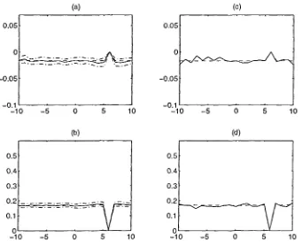
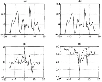
which kurtosis is negative. We use 20 different realizations to study the mean and variance of these indexes. In first place, we observe their behavior for moderate SNR. Thus, fig. (4.8a) and (4.8b) show the estimation for SNR 15 dB, the pixels of the signal are uncorrelated and the Gaussian noise follows an AR model with am =<7jt = 0.8. Each figure shows: in solid line, the mean of the cost function using 20 realizations of a sequence of two (a) 0.05 0.05 0.1 10 0.5 0.4 0.3 0.2 0.1 10 5 5 0 (b) 10 10 0.05 0.05 0.1 10 0.5 0.4 0.3 0.2 0.1 0 10 (c) 5 0 (d) 10 10
Fig 4.8 Cost functions for SNR = 15 dB of a 256 length object where df,°=6; a)
b)J2[;(d) c) single realization QÏ J41^(d) and d) single realization of J2¡.(d)
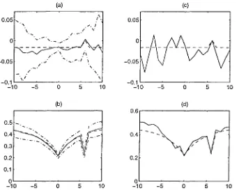
[image:21.568.113.454.332.610.2]estimation for a single realization. The mean estimation is close to the theoretical expectations. The kurtosisbased measure seems to have a higher variance. This fact can be confirmed for lower SNR. Figures (4.9a) and (4.9b) show the mean estimation for both cost functions as well as the mean plus/minus standard deviation when SNR = 2.5 dB (this SNR was chosen since it is close to the theoretical limit to obtain an absolute minimum using the secondorder based index, which is 2.3 dB for these parameters). Clearly, although the mean estimation of the kurtosis tends to the theoretical result the variance is too high. Figure (4.9c) And (4.9d) show the estimation for a single realization. A better way to compare the variance is obtained normalizing both cost functions by their respective mean estimation. Thus, using the same scaling we appreciate in fig. (4.10a) and (4. lOb) the normalized cost functions for low SNR (2.5 dB) and in fig. (4.1()c) and (4. lOd) for high SNR (15 dB). These results suggest that the kurtosisbased cost function should not be used for low SNR unless dealing with longer signals which would reduce the variance. We must be aware of the fact that we are going to use this cost functions for image regions or blocks and the number of pixels may not be large. (a) 0.05 0.05 0.1 10 5 0 (b) 10 0.5 0.4 0.3 0.2 0.1
10 5 5 10
[image:22.569.107.460.390.667.2]0.05 0.05 0.1 0.6 0.4 0.2 (c) 10 5 0 (d) 10 10 5 0 10
Fig 4.9 Cost functions for SNR = 2.5 dB of a 256 length object where dk°=6, a) J4Ik(d) b)
(a)
-10 -5 O 5 10
(b)
2
-10 -5 O 10
(C)
-2
-10 -5 O
(d)
2
-10 -5
10
10 Fig 4.10 Normalized cost functions of a 256 length object where d¡,o=6, a) W2k(d) for SNR = 2.5 dB , c) J41k(d) and a)J2k(d) for SNR = 75 dB
and
A
Modified Kurtosis of the DFD
As we have shown in the previous section, the kurtosis is a very sensitive measure and we need long data records to obtain low variance estimates. On the other hand, image information is repeated along the sequence as it is established in the Intensity Constancy equation, Eq. (4.2). This redundancy may be used to obtain belter estimates of the higher order statistics to reduce the effect of additive noise. Amblard et al. [1993], proposed an adaptive scheme for the estimation of fourthorder cumulants for transient detection. It was proven for the case of i.i.d. random variables that the estimator is asymptotically unbiased. Using this approach, we derived the equivalent expression for the kurtosis of the displaced frame difference which at time k becomes:
Kk (DFD(d))) =Kk.j (DFD(d))+y[ k(DFDk(d)) Kk.j (DFD(d))], A
where k (DFDjJd))) is the "instantaneous kurtosis" given by,
2
k (DFDk(d)) = DFDk(d)3fj DFDk(d) $., {DFD(d))J, (4.32)
and
Ek{DFD2(d)) =Ek.! (DFD2(d)}+ß [jj %DFDk2(d)Ek., fDFD2(d))J, (4.33)
¡i and 7 are forgetting factors that adapt the estimation to changing conditions. The sub index k has been suppressed in the DFDs where previous frames are involved. This adaptive scheme leads to consistent estimates of the kurtosis of the DFD.
Nevertheless, we are interested in obtaining the displacement vector at time k and this only depends on the instantaneous kurtosis, that is, Eq. (4.32) and (4.33). It is clear that there is no information on the current displacement between two frames in previous images or in previous displacements (unless we were dealing with some kind of prediction or motion model). Previous frames can be used to obtain information on the statistics of the regions and/or statistics of the noise. Our goal is to define a low variance cost function which should be, at the same time, asymptotically unaffected by conelated Gaussian noise. One possible solution is based on the instantaneous kurtosis defined by Eq. (4.32), which is normalized to the square of the variance:
/i{DFD2(d)) ] (4.34)
For ¡i =1 only the previous DFD intervenes, and therefore, only three frames are included:
d) (4.35)
mei2m
For small values of ¿í past frames become more significant than the previous one. Thus,
A .7
depending on the estimation of E¿,_j¡DFDz(d)), different versions of the above cost
function may be derived. Observe that instead of having the instantaneous secondorder moment estimate to the power of two, which may show a high variance, we have a term whihc is the product of the instantaneous secondorder moment by the estimated second order moment using more than two frames.
An alternative estimation is necessary in case only two frames are available or when the first two frames of a sequence are not static. In this case, it seems reasonable to use the kurtosis cost function as it is defined in Eq. (4.17) and normalize by the square of the variance. Another approach that we propose using Eq. (4.34) with:
Ek.!{DFD2(d)) > ¿ ^lgkl(m) gkl(md) ] 2, (4.37)
mtfiin
is given by:
J43k(d) = y^— [ft 2k m£U,n
(4.38) The resulting cost function will display a behavior similar to the one in Eq. (4.35), yielding to better estimates of the displacement.
To study these cost functions we derived also the moments of the DFD as a function of signal and noise moments. The development is shown in Appendix D for J 42^), when ß= l, and for J^j^d), where we substitute the summation by the expectation operator. The results are illustrated in the following sections.
The first step is to decompose J 42^) in signal and noise differences. Thus, we obtain their contributions (Appendix D):
J42k (d)= r4^ {E{DSDL4(d))3E{DSDL2(d)}E{DSDk.i2(d)} J 2k (d)
3E{DNDk2(d)}[ EfDSDk.J2(d)JEfDSDl2(d)JJ } (4.39)
which for n=l leads to the expression (Appendix D):
J42km(d) = f — í — /
3/2 cr/ 2rj(dk°d) ] [2(J2 2rjidk.i°d) ]
This is the general expression of the newdefined cost function as a function of the signal and noise moments. Analogously as we did for the previous cost functions, analytical expressions may be derived for the case of correlated and uncorrelated signals.
4.4.1 Study for Uncorrelated Region and Colored Noise:
In this case we obtain:
J42k(d) = v
6cff
Although noise is affecting the behavior of the cost function it does in an appropriate manner. The cost function is characterized in three different areas. In the first one, when the displacement variable is different from the correct current and previous displacements, we obtain the normalized kurtosis which sign depends on the sign of the region kurtosis. When the variable is equal to the current displacement, the value of the cost function is negative. Finally, for the previous displacement, we obtain a value which is higher than the normalized kurtosis. Thus the usual shape of the cost function will show a maximum at the previous displacement and a minimum at the correct displacement. This will be better seen in the examples.
4.4.2 Study for Correlated Region and Colored Noise:
The analytical expression for the case of 1D correlated signals is the following:
2mf4+6fmf4 (bm) af4 (bm af4] ,ddk°) 4 rf(bm ,ddk°)
where the moment functions were obtained in Sections 4.2 and 4.3 for AR models. It is not obvious to recognize what is the behavior of JJ42¡¿d) for different displacements. From Eq. (4.40) we can notice that there is a noise term that multiplies a difference of displaced signal covariances. Thus, if the optimal displacements at time k and k1 are equal, we can easily deduce that J'42^) is nothing else than the normalized kurtosis of the DFDk(d). For other
situations, the following examples will clarify what is, in general, the behavior of this cost function.
Example 4.2 : We either assume the signal is uncorrelated or follows an AR model which input is an i.i.d. sequence uniformly distributed. We use the coefficients am =o¿= 0.6 for
the noise and btn = 0.9 for the signal, the SNR is set to 0 dB. Figures (4.lla) and (4.lib)
show J42i/d) for an uncorrelated and a correlated signal respectively. The displacement is
df.° = 8 and d^f =0. We observe that there is a minimum at the correct displacement and a maximum at displacement zero. As we pointed out, the noise is affecting J42^) in an advantageous manner. Figures (4.1 le) and (4.1 Id) show the theoretical behavior of J42¡(d)
for an uncorrelated and a correlated signal respectively when d^f — d¡P. For this case, the cost function behaves as the normalized kurtosis. It displays a maximum at the correct displacement when the region has negative kurtosis and a minimum when the region kurtosis is positive. The minimum we obtain at displacement zero is due to the normalization factor, the square variance estimate.
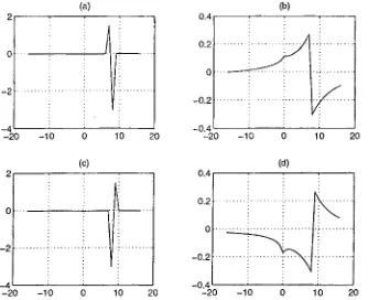
We also study the situation when the displacement changes slowly along the sequence. Figures (4.12a) and (4.12b) show ^¿^ when dk° = 8 and d^¡° =7. As expected, we
obtain a maximum at the previous displacement and a minimum at the current displacement. The same thing occurs when dk° = 8 and dj._j° =9, see fig. (4.12c) and (4.12d). However
we perceive a local minimum at displacement zero which is caused by the noise covariance. This could lead to incorrect results for other AR parameters and different SNR. Fortunately, we have observed that this only happens for extremely low SNR. For white signal this problem does not happen at all.
(a) (b)
-20 -10 O (c) 10 20 O 1 " -10 O (d) 10 20 0.01 0.02 -0.03 -0.04 0.01 0.02 0.03
-20 -10 10 20 0.04-20 -10 O 10 20
Fig 4.1 1 J42i¿d) for a negative kurtosis region a) uncorrelated signal df,° = 8 ,
b) conelated signal, c) uncorrelated signal d¡9 = dk„f, d) correlated signal.
(a) (b)
2
4
-20 -10 0 10 20 (c) 0.4 0.2 0 0.2 0.4 20 10 2
41—
20 10 10 20
0.4 0.2 0.2 -0.4 0 (d) 10 20
-20 -10 10 20
[image:28.568.113.451.89.362.2] [image:28.568.115.449.423.695.2](a)
2
-20 -10 O (c)
10 20
0.4
0.2
-0.2 -0.4
(b)
20 10
2
4'—
-20 -10 10 20
0.4
0.2
-0.2 0.4
O (d)
10 20
-20 -10 10 20
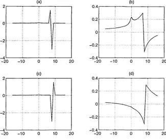
Fig 4.13 JT42k(d) for a positive kurtosis region a) uncorrelated signal d f.0 = 8 , dk_j° = 7,
b) correlated signal, c) uncorrelated signal dk° = 8, dk_¡° = 9, d) correlated signal.
We can then conclude that the newdefined cost function exhibits always an absolute minimum at the desired displacement for positive kurtosis regions. The same behavior is observed for negative kurtosis regions except when dk_j° = dk°, in which case the cost
function becomes the normalized kurtosis. In this situation, the extremum at the desired displacement becomes a maximum. Hence, except for this case, in all other situations the correct displacement is derived from an absolute minimum. We need to introduce a mechanism to avoid searching a wrong minimum when d^¡° = dk°. One approach is to use
¡J.<1, thus, the influence of previous frames allows to keep a minimum at the desired displacement. If this situation stands for many frames we end up in the same situation. An
A 2
additional step is added which consist of introducing a shift of d^f to E¡,.j{DFD¿(d)).
A
Thus, in the following iteration, k(DFDk(d))) will have a maximum atd=0 and a minimum
[image:29.567.117.442.91.364.2]Next we present some examples where we compare the three cost functions defined up to this point. We will see the effects of the estimation and the advantages of using the newly defined cost function. We also test the above procedures for the case ofd/.^0 = djP.
Example 4.3 : In this example we compare the performance indexes for a white 1D rectangular object of length 256, which is moving along three frames where df,,¡° = 0 and d]P = 8. Noise is simulated using an AR model with amak 0.6 and SNR = 5 dB. As in
example 4.1, we generate the sequence 20 times and obtain the mean behavior of the cost function at time k (we represent in dashed line the theoretical curve; in solid line the mean estimation of the cost function; and in dasheddot line the mean +/ the variance of the estimation). We can observe in fig. 4.14b that the kurtosis cost function does not show the maximum at the correct displacement and exhibits high variance. We have normalized this cost function by J2[? (d) to study if there is any improvement, which does not happen as it is
illustrated in fig. 4.14a. Figure 4.14c shows JT42i/d) using the estimation in Eq. (4.35), that
is for ¡1=1, where only the previous displacement is relevant. For the modified kurtosis the variance is much lower and follows the theoretical results. Thus, this cost function can be reliably used for objects of this size in similar situations. For J2i¿d) in fig. 4.14d the variance is low, but for this SNR the minimum at the correct displacement is not absolute. The limit SNR for these parameters is found to be 2.29 dB from a 1D version of Eq. (4.13). Figure 4.15 shows the cost functions for a single sequence realization. The modified kurtosis cost function outperforms all other cost functions.
In the next step, we compare the cost functions for a highly correlated signal and find there is also an improvement in detecting motion using the new cost function. Figures 4.16 and 4.17 depict the mean behavior and a single realization of the cost functions for a 1D colored rectangular signal following an AR model which parameter is bm = 0.8. The SNR is
2dB and the noise parameters are the same. The limit SNR in this case is 1.49 dB given from a 1D version of Eq. (4.15). J42^) shows a minimum that is easily detected. J2^ shows two similar minima at the previous and current displacement.
Example 4.4 : In this example we compare /^¿M) and J 2^) for a 2D white uniformly distributed object of size 16x16. Colored noise that follows an AR model with an=am=cifc = 0.8 is added to a sequence of three images where the object is displaced
dk_J°=(0,0) and dk°=(4,l) . The SNR is set to 0 dB. The absolute minimum for J2k(d)
minimum for J '42^) is (4,1). We found that for this type of signal and SNR = 0 dB we obtain an 80% of error for J ) versus 10% of error for
Example 4.5 : In this example we study the situation when the displacement changes slowly
along the sequence. The signal and noise parameters are characterized by the same values than in Example 4.3 and the SNR is 2 dB. Figures (4.20a) shows a single realization of Jj2k(d) when dj.° = 8, d^f =7 and d^2° 0. As expected, we obtain a maximum at the
previous displacement and a minimum at the current displacement. This situation is
A ,
improved when ¡i = 0.89 in the recursive estimation of E¡<_j{DFD¿(d)) as it can be seen in
fig. (4.20c). The same comments are valid for the case of df.° 8 , d^_f 9 and dk_2° = 0, see fig. (4.20b) and (4.20d).
Example 4.6 :We also compare the tracking capabilities with the ones of J2i/d) using the
A y
procedure to center E^.jfDFDfd)) at dk_j and using ß = 0.89. We are given 10
realizations of a sequence of 7 synthetic noise free images containing an uncorrelated 2D rectangular object. The object was previously segmented and was moving (3,1) pixels per frame. Colored Gaussian noise was generated from a first order AR model with an=am=ak
= 0.6 and added to the sequence. For this size and signal distribution, the cost function J41ffd) did not work at all. Table 1 shows the percentage errors to reach the final position
0.5 (a)
*. /
0.5 !
20 10
'•/, V x '..' »v ' V : *
2
i
0 1 2 20 10 0 (c) 10 20 0.4 0.2 0 0.2 0.4 (b) 20 10 10 20 0.8 0.7 0.6 0.5 0.4 0.3 20 10 0 (d) 10 20 10 20Fig 4.14 Estimated cost functions when dk_j° =0, dk° =8 and SNR = 5 dB for a white
signal of length 256: a) J^j^d) normalized; b')J4If.(d) ; c) J^d) ; d) J2fJ[d)
(a) 0.5 0.5 0.4 0.2 (b) 20 10 0 (c)
10 20 0.220 10
1 0 1 2 20 10 10 20 0.7 0.6 0.5 0.4 0.3 20 10 0 (d) 10 20 10 20
Fig 4.15 Cost functions for a single realization when d¡,_¡0 =0, d
k° =8 and SNR 5 dB for
[image:33.570.110.447.431.703.2]0.4 0.2 O 0.2 0.4 0.6 (a)
-20 -10 O
(e) 10 20 0.5 O -0.5 1 1.5 2 (b) -20 -10 1 O 1 2 3
-20 -10 10 20
2.5 2 1.5 1 0.5 20 10 O (d) 10 20 10 20
Fig 4.16 Estimated cost functions when dk_f =0, dk° =8 andSNR = 2 dB for a colored
signal of length 256: a) J41]¿d) normalized; b) J41k(d) ; c) J42ifd) ; (a) 0.4 0.2 0 -0.2 -0.4 0.6 20 10 2 1 0 _1 2 0 (c) 10 20 0.5 0 0.5 -1 -1.5 2 (b) -20 -10
20 10 10 20
2.5 2 1.5 1 0.5 -20 -10 0 (d) 10 20 10 20
(a) (b)
Fig 4.18 Estimated cost functions for a 2D white object of size=16xl6 where dk_1°= (0,0),
dk°= (4,1), SNR = OdB from 20 runs a) 3D view of J42k(d) ; b) J2k(d) ; c) image view of
J42k(d) ; d) J2t(d).
(a) (b)
Fig 4.19 Estimated cost functions for a 2D white object of size=16xl6 where d^f (0,0), dk°= (4,1), SNR = OdB for a single realization a) 3D view of J42k(d) ; b) J2]¿d) ; c) image
(a) (b) 0.5 O 0.5 1 1.5
-20 -10 O 10 20
(c)
1
2
-20 -10 O 10 20
0.5 O 0.5
1
-1.5
-20 -10 O 10 20 (d)
1
—2
-20 -10 O 10 20
Fig 4.20 J42k(d) when dk.2° = O a) \L = 1 dk° = 8, dk,f = 7, b)/z = 1 dk° = 8, dk.f = 9, e)
// = 0.89 dk° = 8 , dk.j° = 7 d)fj = 0.89 dk° = 8, dk.j° = 9.
size
SNR
J42k(d)
J2k(d)
4.4.4 Simple Versión of the Modified Kurtosis of the DFD
The modified kurtosis cost function displays an outstanding behavior specially when d/f is different from d^f or, in case these displacements are similar, when we center the update or use fi<l. The main improvement is that J r42k(d) exhibits a low variance as compared to
the kurtosis cost function, allowing smaller size signals or regions. On the other side, this new cost function is able to obtain the correct displacement when the SNR is low and secondorder statistics of the DFD lead to ambiguous results. We are interested in defining a cost function with the characteristics of 342^d) even though only two frames are available.
This could be achieved if we replace EfDFD^^d)} for a convenient function. We choose the square differences of one of the frames with the same frame shifted d. The resulting cost function shows a behavior analogous to J '42^) when dk_}°=0, that is, a maximum at
displacement zero and a minimum at the current displacement. It was defined in Eq. (4.38) and we repeat it here for convenience.
gkl(md) ] 2
As we did for the other cost functions we have developed Jjyjd) as a function of signal and noise moments, obtaining (Appendix D):
J43k(d)= ,.,
J 2k (d)
{2wf4+6E{fk2(m)fk2(m+dk°d)HE{fk3(m^
3 [2ffn22rnI(d)J 2+6[2af2 2rj(ddk0) ] [2an22rnl(d) ]
3[2af2 2rj{d) +2an22rn0(d) J [2e2 2rj{ddk0) +2an22rnl(d) ] (4.45)
The following examples will illustrate the response of this cost function.
Example 4.6 : In this example ^42^) ant^ ^43k^ are estimated in an analogous scenario
than the previous examples and are found to look very similar. The performance indexes are compared for a 1D colored rectangular object of length 256, which is moving along three frames where d^f = 0 and df.° = 3. For this case we choose a signal with positive kurtosis generated from a firstorder AR system which coefficient is bm =0.8 and which input is a
SNR = 2 dB. We generate the sequence 20 times and compute the percentage of error for each cost function. Thus, we estimated 95 % of error using J2i/d), 100% of error forJ41k(d),
45 % for J42i¿d) and 50% using J4^(d). Figure 4.21 depicts each cost function for a single
realization.
As we just mentioned, we observe that J42k(d) resembles J43k(d). Nevertheless, we have to
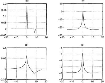
keep in mind that whereas the latter is just an approximation that works correctly up to a certain SNR, the former does not change its behavior for low SNR, like the kurtosis. Figure 4.22 shows the theoretical mean curves for the two cost functions when the SNR is 0 dB. On the other hand when the SNR tends to <», J42¡¿d) does not change its shape while
^43k^ c'oes not snow a minimum anymore, see fig. 4.23.
(a)
100
50
0
-50
-100
(b)
-20 -10 0 10 20
(C)
-20 -10
20
15
10
0
(d)
10 20
-20 -10 -20 -10 10 20
Fig 4.21 Cost functions for a single realization when dk^° =0, dka =8 and SNR = 2 dB for
[image:38.567.103.453.339.637.2](a)
2
_4
-20 -10 0
(b) 10 20 10 -10 -20 30 (c) 20 10 O (d) 10 20 2 4
-20 -10 10 20
2
O
2
4
-6
-20 -10 10 20
Fig 4.22 Theoretical behavior of the cost functions when dk_ f =0, dk° =8 and SNR = OdB
for a white signal a) 342^) ; c) J^d) ; and a correlated signal b) J
0.2 0.15 0.1 0.05 o (a) -0.05 -20 -10 0.1 0.05 o (b) 10 20 10 0 10 20 30 (c) -20 -10 -0.05
-20 -10 10 20
[image:39.566.118.447.86.356.2]1 0 1 2 3 -4 -20 -10 O (d) 10 20 10 20
Fig 4.23 Theoretical behavior of the cost functions when dk,f =0, dk° =8 and SNR =30 dB
[image:39.566.113.453.417.688.2]Example 4.7: The cost function J^^d) has applicability in a different context involving
time delay estimation. Hinich et al. [1989] have shown via bispectral analysis that whereas the ambient ocean noise is indeed Gaussian, the ship radiated noise is nonGaussian. Thus, the use of higherorder statistics for the time delay estimation in passive sonar is well motivated. On the other side, Tugnait, [1991], proposed an optimization approach where the time delay between two signals is estimated by minimizing a mean fourthorder (MFC) criterion, which is nothing else than J41i<(d). To demonstrate its performance he used the
following example. Time delay between two 1D signals has to be estimated. The signal is given by the product/¿.^ (in) = Wk _¡ (m) ßk_](m) where Wk ¡ (m) is Laplace i.i.d and ßk } (in)
is a Bernoulli process. This type of signal is a test signal widely used in the acoustics/ geophysics literature (a lot of controversy exist whether or not it approximates a real signal). The noise sources are spatially correlated, nk_}(m) is generated first, whereas nk(m) is
computed from
10
nk (m) = ]£ b(i) nk1 (m+i) (4.41) 1=0
where b(i) takes the values {0.2, 0.4, 0.6, 0.8, 1, 1, 1, 0.7, 0.5, 0.3, 0.1}. It was seen that J4]l/d) yields the true time delay, that was set to dk°=I6 , whereas J2k(d) does not. The
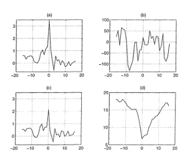
signal length was 2000 and the SNR = 5 dB. In addition, the newly developed cost function J43i/d) can also be used to obtain the true time delay. Figs. (4.24a), (4.24b) and (4.24c)
show the mean plus/minus standard deviation of the three cost functions for 10 realizations. Figures (4.25a), (4.25b) and (4.25c) show the cost functions for a signal of length 64 for 10 realizations. We obtained 90% of error for J4]k(d) versus 20% of error for J42k(d). We can
(a)
20 10 O 10 20
(b)
4
2
O
2
20 10 O 10 20
(c)
2
O
2
20 10 O 10 20
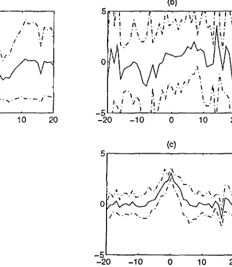
Fig. 4.24 a) mean behavior of J2k(d) for a 1D signal of length 2000 and SNR = 5 dB
b)J41l/d) c)J42k(d)
(a) (b)
ï i> ;n • • • ' •
•J i A ."..'.í''V'l'U.!,! j'. i i \ i!/'' r v
20 10 0 10 20 20 10 O 10 20
20 10 10 20
Fig. 4.25 a) mean behavior ofJ2k(d) for a 1D signal of length 64 and SNR = 5 dB
[image:41.571.117.447.79.369.2] [image:41.571.202.434.418.685.2]Example 4.8: This example demonstrates the improvement of the new fourthorder based
cost function J43k(d) from the secondorder one, J2k(d), when blockmatching is applied to obtain the displacement between consecutive real frames. Figure 4.26a shows one of the original images taken from the "flowers" sequence. Figure 4.26b is the same image when colored Gaussian noise generated from an AR model with ajt = am=an = 0.6 has been added to
the sequence and the SNR is 2 dB. In first place we have manually displaced by (4,0) all pixels in the image. Figure 4.27a depicts the ideal vector displacement map given blocks of 16x16 pixels. The result for noisy frames when using the correlationbased measure is shown in fig. 4.27b. Most blocks are represented by a dot point that indicates that displacement zero has been detected. Figure 4.27c shows the results after applying J^^fd). As a whole, we observe that the detection decision has been improved. Notice that most wrong decisions are located in the upper part of the image where the homogeneous sky is, whereas most correct decisions are located on the flower zone which is a textured region. The percentage of correct decisions for J43k(d) is 17% and 7% for J2k(d). Another important measure of closeness is derived when the difference of the computed from the correct displacement is less or equal than one pixel. Thus, a 37% of closeness is obtain for J43k(d) versus a 7 % for J2k(d).
(a) (b)
(a) (b)
(C)
Fig 4.27 a) Noisefree displacement map given blocks of 16x16 pixels after applying J2k(d),
where all pixels in the second frame have been displaced by (4,0) b) map for noisy frames using J2k(d). c) using J43k(d).
(a) (b)
•s x ' , '
v _ _ _ _"H _
(c)
Fig 4.28 a) Noisefree real displacement map given blocks of 16x16 pixels obtained from
J2k(d). b) displacement map for noisy frames when using J2k(d) c) using J43i¿(d).
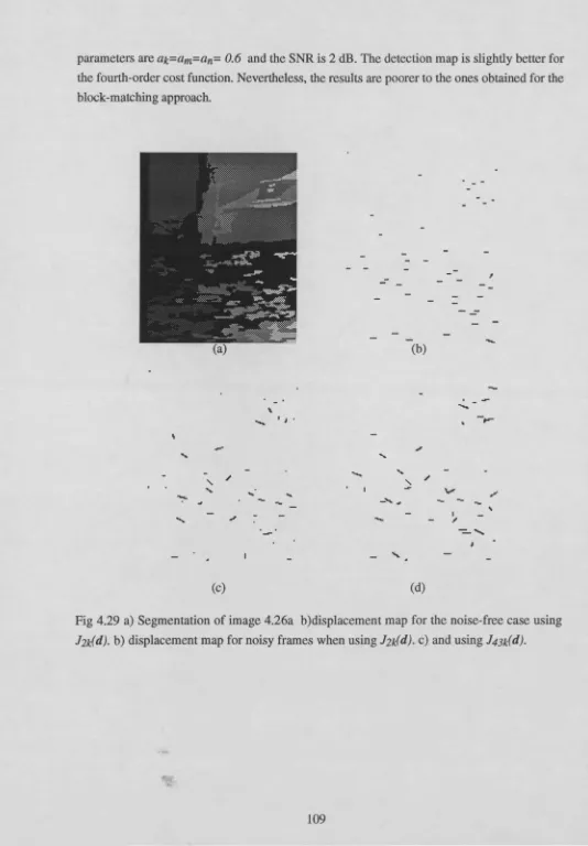
[image:44.571.124.459.96.493.2]parameters are ak=am=an= 0.6 and the SNR is 2 dB. The detection map is slightly better for the fourthorder cost function. Nevertheless, the results are poorer to the ones obtained for the blockmatching approach.
(b)
\
N. \
(c) (d)
Fig 4.29 a) Segmentation of image 4.26a b)displacement map for the noisefree case using
[image:45.552.8.542.26.794.2]