Stability of Controllers with On-Line Computations
PEDRO J. ZUFIRIA RAMESH S. GUTTALU
Abstract. The dynamical systems theory developed by Zufiria [1], Zufiria and Guttalu [2, 3], and Guttalu and Zufiria [4] is applied to the stability analysis of control systems in which the feedback control law requires in real time the solution of a set of nonlinear algebraic equations. Since a small sampling period is assumed, the stability and performance of the controlled process can be studied with a continuous-time formulation. A singularly perturbed system is used to model both the dynamics of the system being controlled and a numerical iterative algorithm required to compute the control law. An updating control procedure has been proposed based on the iterative nature of the control algorithm. The results obtained by Zufiria [1] regarding the behavior of a dynamical system that models the numerical algorithms lead to a considerable simplification in the analysis. For the case of a control problem involving inverse kinematics, the numerical algorithm that solves for inverse kinematics can be considered as an observer (or an estimator) of the state-space variables. The study provides an estimate of the required speed of computations to preserve the stability of the controller.
1. Introduction
Global behavior of a class of dynamical systems of the form
i = - / - ' ( * ) / ( * ) , x € RN, / 6 C\ J{x) = Vxf(x) (1)
has been studied [1-4]. In addition, some discrete formulations obtained by numerically integrating the dynamical system (1) have been considered [1]. These discrete formulations can be represented, in general, as discrete dynamical systems (or maps) of the form
xn+t = G(xn), x € RN, G: RN -• RN, n € Z. (2)
Both types of systems (1) and (2) are typical formulations for determining the zeros of the vector function/ A study of these dynamical systems sheds light on the behavior of some of the standard numerical algorithms employed to find the zeros off. Note that one-step Euler numerical integration of the continuous-time system (1) leads to the Newton method, which is an iterative technique or discrete system of the form (2).
equations in real time. The algorithm that solves the algebraic system is referred to as solv-ing algorithm. A classical analysis of the performance of these given control designs requires that a solution of the algebraic system be determined in negligible real time, without affect-ing the performance of the controller. On the other hand, if the number of algebraic equa-tions to be solved is considerably large or the dynamics of the system to be controlled are last enough, then the dynamics of the solving algorithm should be taken into account. The time taken by the computer to calculate the control law has been considered in the literature on classical control of linear time-invariant systems where pure delay units are used to characterize the computation time (see [5]). The nonlinear case presents two main difficulties. One of them is how to characterize the dynamics of the solving algorithm. The other relates to the combined analysis of the dynamics of the system being controlled and the solving algorithm.
A characterization of the dynamics of algorithms for solving an algebraic system has been developed [1], and continuous-time as well as discrete-time formulations are considered there. In this article, the continuous-time formulation is employed to characterize both the solving algorithm and the system being controlled, based on the following assumptions. First, the sampling period is smaller than the characteristic time of evolution of the dynamics of the system being controlled. In addition, the sampling period should be smaller than or of the same order of magnitude as the iteration time of the numerical algorithm. Finally, the control law is updated for every sampling instant with the iterate value that is being employed in the iterative algorithm at that sampling instant.
If the dynamics of the numerical algorithm are faster than the dynamics of the system being controlled, the combined analysis of both systems can be performed via a singular perturbation formulation [6-8]. The singularly perturbed system can be divided into two subsystems. The first one, called the reduced-order system, represents the dynamics of the system being controlled. The second system, named the boundary-layer system, models the "fast" dynamics of the solving algorithm. Since they are coupled, both systems can be studied simultaneously with the singular perturbation formulation.
The organization of this article is as follows. In section 2, a background of some known results concerning singular perturbed systems is provided. An implementation of a controller requiring on-line computations is presented in section 3. A singularly perturbed system is used in section 4 to model the system being controlled and the on-line controller. The theory developed by Zufiria [1] considerably simplifies the analysis. The results are applied to obtain stability results for tracking control problems. Based on the same singularly per-turbed formulation, some stability results are also obtained in section 5 for controllers requiring computation of inverse kinematics. Examples provided here illustrate the utility of theoretical results. Concluding remarks appear in section 6.
2. Background
Theorem 1. Consider the linear time-invariant singularly perturbed system given by
x = Aux + Al2z, x € RN, z € RM (3)
ez = A2lx + A22z, e > 0 (4)
where An, A12, A2X, A22 are constant matrices of appropriate dimension. If A~\ exists and
if A0 := Au ~ Aii^A2i and^22 a re Hurwitz matrices, then there exists an e* > 0 such
that for all e € (0, e*] the system (3-4) is asymptotically stable.
Note that this theorem only provides information about the existence of values of e that guarantee asymptotic stability of the system. If the system (3-4) is a linear approximation of a nonlinear system at a given asymptotically stable equilibrium point, then no conclu-sions about the associated domains of attraction can be drawn. The following result pro-vides some information about stability and domains of attraction for nonlinear systems (see [6]):
Theorem 2. Consider the singularly perturbed system
i = fix, z), / : RN x RM -» RN (5)
d .= g(x, z), g: RKX RM- * RM (6)
where / and g are smooth enough to ensure that the systems have a unique solution for a specified initial condition. Let Bx C RN and Bz C RM denote closed sets. Let • ( • ) and
$(•) be two scalar functions of vector argument that vanish only when their argument is zero (these are referred to as comparison junctions). Suppose that the following assump-tions are satisfied:
1. The origin is an isolated equilibrium of system (5)-(6) in Bx X Bz, and z = h(x) is
the unique root of the equation 0 = g(x, z) for (x, z) in Bx X Bz.
2. There exists a Lyapunov function candidate W(x, z) such that for all (x, z) € Bx X Bz
the following conditions are satisfied:
a. W(x, z) > 0, Vz * h(x) and W(x, h(x)) = 0 b. (VZW) • g(x, z) < - a2#2( z - h(x)), a2 > 0
c (V^HO -f(x, z) < y$\z - h{x)) + 02*(xMz - h(x)).
3. There exists a Lyapunov function V(x) that for all (x, z) € Bx x Bz satisfies
a. (VXV) -f{x, h(x)) < - a , *2( x ) , a, > 0
b. (VXV) • [f(x, z) - fix, hix))] < &*(x)#(z - Hx)).
Then the origin is an asymptotically stable equilibrium of the singularly perturbed system (5)-(6) for all e 6 (0, e*), where
Moreover, for every number p 6 (0, 1) the function
v(x, z) = (1 - p)V(x) + PW(x, z), 0 < p < 1 (8)
is a Lyapunov function for all e 6 (0, ep), where ep < e* is given by
«ty + ^r^p-^-^ + eM
2(9)
The parameter p defines a family of Lyapunov functions, and its selection may depend on different criteria such as the desired shape of the level curves or the upper bound ep. The
upper bound has a maximum value e* that corresponds with the value p* = /V()3i + (32
)-Based on the Lyapunov function, we can define the set
S = {(x, z) | v(x, z) < c] C Bx X Bz, c > 0, (10)
which is included in the domain of attraction of the equilibrium.
One notes that in the singularly perturbed system (5)-(6), the reduced system corre-sponds to
i = f(x, h{x)), f: RN X RM -» RN (11)
and the fast system corresponds to
ez = g(x, z), g: RN X RM -• RM (12)
where x is considered as a constant because of its slow time variation when compared with that of z for a small enough e > 0.
One can show that the assumptions made in the above theorem are mild and that there is a wide class of systems for which they hold, as shown in the following lemma, which is taken from Saberi and Khalil [7].
Lemma 1. Let/, g, and h be continuously differentiable in Bx = Bz. Suppose that the
reduced system is exponentially stable such that \\x(f)\\ < c3|jx(0)||e~c*r whenever x(0) e Bx.
Let Bx c f i j b e a set for which every trajectory starting in Bx remains inside Bx. For every
x € Bx, suppose that the equilibrium point z = h(x) of the "fast" system is inside Bz and
is exponentially stable uniformly in x such that ||z(r)| < c5||z(0) - h(x)\\e~c,,T whenever
z(0) € Bz. Let Bz c §z be a set for which every trajectory starting in Bz remains inside
Bz. Then the conditions of the above theorem are satisfied in Bx x Bz.
V(x) = (T l|9C(í, x)\\2dt
Jo
W(x, z) = I ||S(T, Z; X) — h(x)\\ dr J o
where T > 0 is an arbitrary constant, SC(i, x) is the trajectory of the reduced system start-ing at an initial point x(0), and Sir, z; x) is the trajectory of the fast system startstart-ing at an initial point z(0). Consequently, the above lemma is mainly of a theoretical value and does not provide a convenient way to determine some values for the constants oti, a2, j3,,
&, and 7.
In the following sections, we will apply the above theorems to a special class of singu-larly perturbed systems that model dynamical systems with control laws requiring on-line solutions of coupled nonlinear algebraic equations. For some cases, one is able to provide practical forms of Lyapunov functions.
3. An "updating control" procedure
Due to the digital nature of practical controllers, one can define a measurement sampling period that defines how frequently measurements are performed (at given sampling instants). These sampling instants usually define also the times at which the control law must be updated. The classical implementation of control laws with on-line computations updates the control value after the algorithm has obtained a new solution for the control value. Hence, this procedure assumes that the control algorithm is fast enough to provide a new control value before a new sampling instant arrives. It is known from digital control theory that the sampling period has to be chosen small enough when compared to the characteris-tic times of evolution of the system and controller dynamics. A problem arises whenever the computation of the control law requires more time than the sampling period.
e = ^ (13)
where TR is the real computer time needed to compute a conceptual evolution time Tc in
the solving algorithm. In other words, e represents the ratio of the real time units of the system being controlled to the conceptual time units of the algorithm.
4. Computed implicit model reference control
In this section we consider control algorithms where the control is defined in an implicit manner so that the system follows a model reference system. Note that the term implicit here refers to the fact that the control law is given in an implicit function formulation. This concept is different from the one in direct adaptive control, where the estimates of the parameters of the system are used implicitly. In direct adaptive control, the expression of the control is given explicitly but not as a function of the estimates of the parameters of the system (i.e., the control law is computed directly without need of a previous explicit estimation of such parameters).
Making use of the singularly perturbed formulation, we now analyze the stability of some of these control algorithms. Consider the system
x = f{x, u), f: RNX RM- * RN (14)
where / ( 0 , 0) = 0. We want x(t) to follow the trajectory of the system given by
x = g(x) (15)
for which the origin is asymptotically stable and there is a positive definite function V{x) for which (VXV) • g < -a^^x), a, > 0, where ^(*) is a comparison function. To
char-acterize the algorithm that computes the control, suppose that
h(x, u) = f(x, u) - gix) (16)
and that there exists a control uix) that is the unique root of h(x, u) = 0 in a given region of study. Note that under this specific definition, we will consider h to be smooth enough (e.g., analytic). Then one can model the algorithm that solves for w*(i) via the evolution equation for « given by
m = -iVuhix, u)ylhix, u) = -(VM/(x, u)y\fix, u) - gix)), (17)
which is of the form (1). The value of e is given by the ratio defined by equation (13), which is the ratio of the real time units of the dynamics of system (14) to the conceptual time units of the algorithm described by equation (17).
4.1. A linearization approach
Ai = Vxf(Q, 0)Ax + V«/(0, 0)Au (18)
&i = -W«f(0, 0)r\Vxf(0, 0) - Vxg(0))]Ax - Au. (19)
Note that
A22 = -I, A0 = Vxg(0). (20)
If the origin of the reference system (15) is exponentially stable, then by the definition of g(x), A0 and A22 are both Hurwitz matrices. Applying theorem 1, we deduce that the system
(18)-(19) is asymptotically stable for small enough e.
Note that when the perturbed system is very close to the solution (x = 0, u = 0) the model (17) of the numerical algorithm (fast subsystem) reduces to a linear exponentially stable system that has an eigenvalue of - 1 with multiplicity N. Theoretically, this system would take infinite time to reach the equilibrium point.
In practice, a numerical implementation is suitably modeled by a discrete system. Some of the discrete forms applied to this linear system can provide convergence in a finite number of steps (e.g., in one step for the case of Euler one-step integration representing the stan-dard Newton method). Then the rate of convergence of the algorithm is not very well modeled by a continuous-time formulation (in feet this would correspond with the case e = 0, because only one iteration is needed). This is another aspect that limite the applicability of the lin-earization approach.
4.2. A nonlinear system approach
Equations (14) and (17) define a nonlinear singularly perturbed system. Based on theorem 2, suppose that #(•) is another comparison function and that the following assumptions are met for a given control u{x):
-2hTh < -O>2$2(K - «*(*)), a2 > 0 (21)
2hT(Vxh) • / < 7$2(« - u(x)) + ¡32f-(x)$(K - u\x)) (22)
(VXV) - h(x, u) < P^ixWu - u\x)). (23)
Then the controller guarantees asymptotic stability of the origin for equations (14) and (17) provided that the solving algorithm represented by equation (17) is fast enough so that e € [0, e) where e* is given by equation (7). The Lyapunov function for the entire singu-larly perturbed system has the form
v(x, u) = pV(x) + (1 - p)hT(x, u)h(x, u), 0 < p < 1.
Note that the whole set of conditions of the theorem for nonlinear systems reduces to three simple ones, as stated in assumptions (21)-(23), for this case.
the system (17) are defined by det(VJiT(x, «*(*))) = 0. One may think that these manifolds
may appear in the region of study and hence may jeopardize the results obtained above. The following lemma proves that this is not the case and strengthens the validity of previous results when $(•) can be approximated at the origin by a linear term. In all the problems considered in this article, #(•) is chosen to be either a linear function or a norm function (which behaves like a linear function).
Lemma 2. Suppose that $>(•) can be approximated at the origin by a linear term. Then,
condition (21) is satisfied in a neighborhood of the origin if and only if no singular manifold is present.
Proof. Consider the Taylor expansion around u = u{x):
-2hTh = -2((« - u(x)f(Vuh(x, u(x)))TVuh(x, u(x))(u - u(x))
+ 0(||« - «*(*)||3).
For assumption (21) to be satisfied, it is required that
(V„/i(x, u(x)))TVuh(x, u(x)) > 0,
which implies that det(Vuh(x, u*(x))) ?* 0. Conversely, if det(yji(x, u(x))) ^ 0, then hTh
grows quadratically and assumption (21) is satisfied for small enough a2 > 0.
This result indicates that az is a critical constant in the sense that for a2 > 0 to be satisfied,
the analysis must be restricted to a region where no singular manifold exists. In addition, the value of e(a2) represents a tradeoff between the size of the region where theorem 2
is applicable and the requirements to be met by the fast subsystem parameter e. The larger the region, the smaller the parameter e (or faster the subsystem) must be.
4.3. Example 1
To illustrate results obtained so far, consider the following control problem
x = u + (1 + u*)x, x 6 R, u 6 R (24)
Where we want the system (24) to follow the reference system
x = g(x) = -x, J : Í R . (25)
Note that it is difficult to obtain an analytical expression for the control law. Then the equation determining the fast subsystem is given by
4.3.1. Linear approach. A linearization of systems (24)-(26) in the neighborhood of the
equilibrium x = 0 and u = 0 gives the linear time-invariant (second-order) singularly per-turbed system
Ax = Ax + Au
eAw = —2Ax — A«
whose eigenvalues are
K2 = ¿ (-(1 - «) ± V(l - ey^Ae ] . (27)
The linearized singularly perturbed system is asymptotically stable for e < 1. This pro-vides an upper bound on e but no information about the domain of attraction associated with the origin x = 0 and u = 0 of the original nonlinear system (24)-(26).
A delay model is employed in the classical analysis of the influence of computer time on the control of linear time-invariant systems. Suppose that the computer takes a time T to compute the control law. The transfer function of the whole system and controller would be
Tf= s- 1 +2e~'T' ( 2 8 )
which, via a Nyquist plot, implies that the system becomes unstable for T > ln(2) « 0.7 second. In order to compare this absolute time result with the bound on the parameter € obtained with the approach presented here, we need to explicitly take into account the computational details (method, computer features, etc). Suppose that the computer deter-mines the control law via an iterative method that is modeled by the form (1) and that the sampling period is small enough. If the initial iterates are close to the solution, then the linear model can be considered as valid. The classical result obtained from a Nyquist plot would require the computer to find the roots (exact control law) in less than 0.7 second. On the other hand, suppose that we update the control with the current value of the iterate at every sampling instant whether or not a convergence to the root is achieved. Then, the stability of the origin of the total system (24)-(26) is guaranteed if the computer calculates the iterations equivalent to one logical second in less than one second of real time.
Note that, in the classical Newton method (with unit step size), one logical second cor-responds to one iterate of the algorithm (that is, one iteration of the map (2)). Nevertheless, when the linear approximation is considered, the continuous-time model does not quite represent the time evolution of the algorithm. This is so because Newton method applied to a linear system converges in one iteration as opposed to the exponential decay of the continuous-time system.
4.3.2. Nonlinear approach. More refined results relating the value of e with the domain
steps defined in theorem 2. After some algebra, we obtain the following quantities defined in that theorem:
Bxx Bu = [-0.338, 0.338] x [-0.88, 0.88]
W(x, u) = (xu4 + u + 2x)2
*(y) = Hy) = y
\4u3x\\ < 1 , 0 < <x2 < 2
7 = 2(2 + 0.882)
¡32 = 2(2 + 0.882)
0i = 2
= 5.55 2
-= 5.55 2
a2 a2
2 - 11.09 2 - a2
4(2 + 0.882)
0.2649.
Here 0 < a2 < 2 is to be chosen. The singular manifold of the fest subsystem is defined
by the equation 1 + 4u3x = 0 for a2 = 0. For a fixed value of a2, we obtain an associated
domain of attraction where asymptotic stability of the solution is guaranteed if e < e*(a2).
Figure 1 shows the solutions of h(x, u) = 0, which provide an ideal control law u as a function of the state x, For each value of x, up to four possible solutions for u may exist. Two of these appear in continuous and dashed lines, respectively, within the region of the figure. Figure 2 shows the regions of stability as defined in equation (10), which are delineated by the Lyapunov level curves. The estimates of the domain of attraction are delimited by Bx x Bu and parameterized by a2. The dotted line corresponds to a2 = 0.2, the dashed
line to a2 = 1.0, and the dashed-dotted line to a2 = 1.8. The line defined by the symbol
"*" represents singular manifolds.
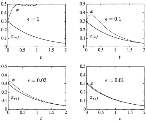
Simulation results for different values of e are shown in figure 3 for initial conditions x(0) = 0 . 3 and M(0) = 0.8. It can be seen that if e > e*(a2), asymptotic stability is not
guaranteed and the system can become unstable. If e < e*(a2), asymptotic stability is
u
Figure 1. Solution curves for example 1.
5. Control based on inverse kinematics
The updating control law developed earlier and the results on singularly perturbed systems find potential application in control problems dealing with inverse kinematics. Consider the problem of controlling a mechanical system described in the form
§ = f(0, u), u = u(6), / : RN X R M RN (29) where a stabilizing control law in the form u = u(0) is provided. The main difficulty here is in obtaining the values of the feedback law «(•)• This is due to the fact that 0 is not directly measured; instead, a related variable x is measured. In general, the kinematic rela-tionship between coordinate variables is defined implicitly by
g(d, x) = 0, g: RN X RN R* (30)
Suppose that we define a solution of equation (30) in the form 0 = 6(x). Then, one can define the following system in terms of the variables x and u:
i = h(x, u) = (Vxg(6(x), x))_1V9g(e(x), x)f{0, «), h: RN X R! M R* (31)
Figure 2, Level curves of the Lyapunov function V(x) as a function of a2 for example 1.
Without loss of generality, we suppose that 9 = 0 is an equilibrium point of system (29) and that this corresponds to x = 0 in equation (30) so that g(0, 0) = 0. Note that while the measured vector is x, the control is defined in terms of 6, which is a vector of joint coordinates. Suppose that there exists a control law u = u(6) that makes the origin of system (29) an asymptotically stable equilibrium point. Then, the corresponding point xe = 0 and
g(0, xe) = 0 will also be an asymptotically stable equilibrium point of system (31) under
the control law u = u(6(x)) = u(x). To characterize the algorithm that computes the con-trol law, we define 6(x) as the unique root of equation (30) for a given measurement x in a specified region of study (i.e., a neighborhood of 0 = 0 and x = 0). Then, an iterative algorithm to solve for 6(x) can be characterized via an evolution equation for 6, the estimate of 6(x), given by
6§ = -(Vjg&x^g&x). (32)
0.5
0.4
0.3
0.2
0.1
0
"—'" I"~
. X
V N.
. &ref
e
-N
1 1 1
-0.1
0 0.5 1 1.5
t
Figure 3. Simulation of trajectories of example 1 for different values of t.
0 = f(0, u(0))
el = -Vestí, x(0Wl8(l x(0))
or as
i = h(x, u) = (Vxg(0(x), x)r%g(0(x), x)f(0, u(§)),
¿ = -(V§g(0, x)Txg{0, x).
(33)
(34)
We consider a region of analysis where a diffeomorphism between 0 and x is defined implic-itly by equation (30).
5.7. Linearization approach
The linearized form around 0 = 0 and 0 = 0 of the formulation given by equation (33) is
eA0 = -<ySg(0, x(0)y1Veg(0, mw - A0 (36)
for which we obtain A0 = Vs/(0, u(0)) and A22 = —1, both of which are Hurwitz matrices
whenever the control stabilizes the origin of the mechanical system exponentially. Hence, for small enough e, the singularly perturbed system will also have an asymptotically stable equilibrium point.
5.2. Nonlinear approach
In order to obtain some information regarding the domain of attraction associated with the equilibrium point, we need to use the nonlinear approach. For definiteness, consider the formulation given by equation (33). Suppose that there is a positive definite function V{0) satisfying (7eV) -f(0, u(6)) < -a^2(0), at > 0. The same can be concluded about
formulation (34) by considering the implicit function theorem and regular partial derivatives of g at x = 0 and u = 0. Then, there exists a positive definite function V(x) satisfying (VXV) • h(x, u(x)) < -a{$\(x), a¡ > 0, where "*"i(*) is a comparison function. Assume
that $(•) is another comparison function and that, referring to the theorem for nonlinear systems, the following assumptions are met in a neighborhood of the origin in the state-space region Bff x B¡¡:
-2gT(§, x(0)) • g(§, x(0)) < - a2#2( 0 - ff), a2 > 0 (37)
2gT{Veg{0, x(9))) -f(6, u(§)) < 7*2(0 -0) + /32¥(0)*(0 - 0) (38)
<y*v) • me, «(*)) - h{0, u(0))} < ^wme - e). (39)
Then the controller guarantees asymptotic stability of the origin for systems (29) and (32), provided that the algorithm is fast enough so that e € [0, e*) where e* is given by equation (7). The Lyapunov function has the form
v{0, 0) = pV{0) + (1 - p)gT(0, x{0))g(0, x(0)), 0 < p < 1.
The singular manifolds are defined by det {Vgg(0, x(0))} = 0. One can again prove that lemma 2 is true and that the condition give by equation (37) is satisfied in a region where no singular manifold is present whenever $(•) is linear.
5.3. Explicit form of transformation
A general implicit form relating the coordinates x and 0 has been previously considered. We now consider the inverse kinematics problem where the transformation of coordinates is defined as
Here, an analytical expression for the inverse function 0 = A~l(x) is not available. As
before, we can work with either 6 or x as the state variable. If we define a region of study in 0 as Be, then the corresponding region for x is given by
Bx = {x | x = A{0), 0 € Be}. (41)
For purpose of simplification, let the initial guesses be confined to the same region Bu = Be. Suppose that equation (40) is a diffeomorphism in the region of study Bs X B§.
Then, there is a unique relation between the two sets of variables 0 and 0 defined by g(§, x(6)) = 0 and the first condition of theorem 2 is satisfied. Let
g(0, x(6)) = A(0) -x= A{0) - A(6), (42)
The singularly perturbed system (33) now takes the form
0 = f(0, u(§)
el = -(VeA(§)rl(A(§) - A(0)). (43)
Note that without loss of generality 6 = 0, and 9 = 0 is the equilibrium point of the singularly perturbed system. For a tracking control problem, one may apply a control law such that xr (or equivalently dr) is the new equilibrium point. In that case, one can define
x
= * -
x
r, e = e -
e
r(44)
x = A(6) (45)
where B¿ or B§ defines a neighborhood around x = 0 or 6 = 0. Note that the Jacobian of the transformation must be analyzed in a neighborhood of xr (or equivalently near 6r).
A linearization approach leads to
A0 = Vef(6, u(0))Ad + V§f(0, u(6))A6
eA0 = A0 - A<? (46)
For a nonlinear analysis, let
J = V,A(0)
K = Véf(6, «(9))
L = VeV(6)
amax(') = Largest singular value
Then the conditions mentioned in theorem 2 can be put in the following form:
Condition 1
-2g(§, x(6)fg(6, x(0)) = -204(0) - A(0)f(A(0) - A(d))
< ~2a2miB(J)\\e - 0||* < -a2&(8 - 0), a2 > 0.
Condition 2
2gT(Veg(d, *(0)))/(0, «(*)) = 2(A(ff) - A(0))TJ(6)f(6, «(*))
= 2(A(6) - A(6))TJ(6)[f(d, u(0)) - f($, M(0))]
+ 2(4(6) - A(6))TJ(6)f(B, m)
* ^ w o ^ a o w o - 011
2+ 2crmax(/)||/(0)/(0, u($))\\ • ||0 - 0||
* 2<r2mm(J)omm(K)\\é - 0||2
+ 2 4a x( / ) | | / ( 0 , u(6))\\ \\8 - B\\
< 7$2(# - 0) + |32¥(0)$(0 - 0).
Condition 3
<y9V)lfW, «(*)) - f(B, u($))] = L(0)[-/(0, u(B)) + f(6, u(6))]
< a
maK(K)\\L(e)\\ \\e - ell
< /3,¥(0)#(0 - 0).
Here, a,^') and ffmax(-) are evaluated at a point (6, 6) € Be x B$.
To obtain some bounds (and to satisfy above inequalities), one must find maxima of sin-gular values or related expressions in any pair (0, 0) € Be x B¡:
max 0(0) = max [max O(-), max 0(0)]. (47)
(0,9)€JS9xB¿ kB¿ OíB„
Here, 0 is any expression to be maximized (e.g., a singluar value of a matrix). If the region B% is chosen equal to Be, then the maximization problem reduces to one variable. Hence,
a2 = 2 mm(eMBeXB. amin(./) = 2 m i n ^ . «^(/(fl))
7 = 2 m a x ^ . (aLx<7)<W(70)
ft = 2 max¿€B. <4«<7)
ft = maxe-€B¿ amax(ÜD
„ - m i n min[ll¿(g)H, l[/(g, ii(fl))H] _^ min[|l¿(fl)|l, H/(fl, «(g))||]
««*» max[||L(0)||, 11/(0, a(0))||] fcty max[||L(0)||, ||/(0, w(0))||]
We also define the functions $(0) and ¥($) to be
*(0) = Hell
*(0) = max[||L(0)||, ||/(0, M(0))||]
such that ^(0) for 6 € Be satisfies
¿LAJ)\\f<0, "0))ll * 0
2*0)
<rmaxWl|L(0)|| < ft*(0)
L(0)/(0, «(0)) < -Ul**0)
and the region of validity (0, 0) € 59 x fig is determined by the value of a2- Notice that
$(•) increases linearly, and for a2 > 0, no region with singular manifold can be included.
This ratifies the results of lemma 2. The Lyapunov function is given by
p0, 0) = pV(9) + (1 - p)(A{6) - A0)f(A(6) - A(d)), 0 < p < 1 (48)
and the level curves are in general (2N — 1) dimensional manifolds defined by v(8, 0) = c > 0, which can be located by employing the singular manifold algorithm provided by Zufiria [1]. One can successively check the level curves v(0, 0) = c associated with different values of c and find the curve with the highest value of c that can be included in B0 x B§. Alternatively, one can calculate the minimum of c on the boundary of the
region of study via a nonlinear programming algorithm. In order to get estimates of domains of attraction, we choose sets as defined in equation (10).
5.4. Example 2
Consider the two-link robot arm shown in figure 4. Suppose that an arbitrary torque is applied at each of the joints. We define the following two related sets of state-space variables:
X\
x3
- * 3 _
= Xi X2
x3
X4
, e
=
r^
1
« ie
3L ^3 J
=
r ^ l
62
03
L M
(49)
The dynamics including the control are given by (see [9])
hH33e24 + 2hH„0A ~ ffsaGi + hHl36\ + Ht3G3 + H3iUl - Hl3u2
-hHue\ - HnG3 - hHue\ - 2hHl362e4 + ff13G, - Hl3ut + Hnu2
where the control vector u represents the torque applied to the joints and
Hn = mj2cl + /, + m2[l\ + 1% + Wo. cos 03] + I2
H33 = m2l2c2 + h
HX3 = m2lrlc2 cos 03 + m2l2c2 + h
Ha = Hn + H33 + H\3
h = m2lxl2 sin 63
Gi = mJd cos 0, + m2g[lc2 cos(0i + 03) + l¡ cos 0,]
G3 = m2lc2g cos(0x + d3).
A simple control can be defined as a function of the joint angles and velocities. This con-trol law is chosen to cancel nonlinearities and to follow a prescribed reference path dm
and $3R. It is given by
Ul = -M\ - 2 A 0 A + G, + ^ i [*,(0, - dm) + k262]
+ ^ r
1[k
3(e
3- e
3R) + k
4e
4]
u2 = h»\ + G3 + ^ ^ [fc,(0, - *i*) + M J
ft, fe(03 - #3*) + *A]
where flj, = Hu + H33 - H\3 and k¡, i = 1, 2, 3, 4, are constants to be determined.
Therefore, the dynamics of the controlled system are given by
01 = 02
02 = *,(0, - 0IK) + fe202
04 = *3(03 - 03fi) + * A
-Suppose that only displacement and velocity of the end of the arm are measured. The kine-matic relation between the variables 0 and x is given by
x = A(6)
where the transformation function A($) is given by
(50)
AW =
lx COS 0, + l2 COS (0j + 03)
- / , 02 sin 0j - /2(02 + 04) sin (0, + 03)
h sin 0, + l2 sin (0, + 03)
/,02 cos 0, + l2(d2 + 04) cos (0, + 03)
Here, the controller must solve for 0 as a function of the measured vector x. The general structure of the whole system is shown in figure 5. Hence, for the analysis, one can employ the singularly perturbed system formulation given in equation (33). The region of evolution B§ X BB must be chosen so that the conditions for applying the theorem for nonlinear
sys-tems are satisfied. From the conditon of uniqueness of the solution, it is easy to check that the range of variation of 03 must satisfy 0 < d3 < w or - -w < 03 < 0. Also az > 0
must be satisfied. Lemma 2 requires that no point with singular Jacobian VeA(0) be
in-cluded. After some algebra, the determinant of the Jacobian is given by
det(VeA(0)) = l\l\ sin2 93 (52)
Hence, we again conclude that the region of study must be a subset of either the region
B§ = Be C {(x, 0)|O < 03 < x]
or the region
Bg = Be C {(x, 0)| - x < 03 < 0}.
In addition, one may expect that stability may also depend on the velocity of the arm and some limits must be imposed on the range of values attainable by 02 and 64. For example,
let us choose two regions of study in the form
B§ = Be = {$ | - 0.5 < d2 < 0.5, 0.3TT < 03 < 0.7», - 0.5 < 04 < 0.5}
and
B§ = Be = {0 | - 1 . 0 < 02 < 1.0, 0.2» < 03 < O.STT, - 1 . 0 < 04 < 1.0}
XR(t) A~l(.)
M0 +,
>
-6{t)
Control
U(B)
—* f(6,U)
Real time
A- '(•)
9(t) >. A(.)
X (t)
where - T < 6X < T for all the cases. Let the physical parameters be
ml — m2 = 1 Kg, lt = l2 = 1 m
hi = kz = 2 m' 7i = 72 = 12 ^ ' m 2
and the control law parameters be
kt — k3 = —1
k2 = ¿4 = —2
so that
K0) = (0 - eR)TP{B - eR)
H
0 0
= (e - e,)7
i i 2 2
0 0
0 0 0 0
3 1 2 2
1 1 2 2
(» - »*). (53)
After some involved algebra1 one can obtain analytical expressions for /, K, and L. A
non-linear programming approach has been employed to obtain the values of the constants au
«2, A> 182, and 7. The value of c that determines the highest-level Lyapunov curve that can be fitted in the regions of study is obtained by calculating the minimum of the Lypapunov function on the boundary of the region of study, also making use of a nonlinear program-ming algorithm. The parameter values obtained for the two different regions considered are shown in table 1. For the case when 9R is a function of time (i.e., the problem of
track-ing a given trajectory), we impose that $R(t) € Be so that the state variables of the system
will remain in the region of study. In addition, the maximum value of the constant c that one can choose in equation (10) depends on 6R. In order to guarantee stability of the
track-ing problem, we choose the minimum of all the possible c values when dR(t) is restricted
to evolve within a given region. Table 2 shows different values of c obtained for two dif-ferent regions where —T/4 < Bm(t) < T/4 and $3R(t) is allowed to evolve. To preserve
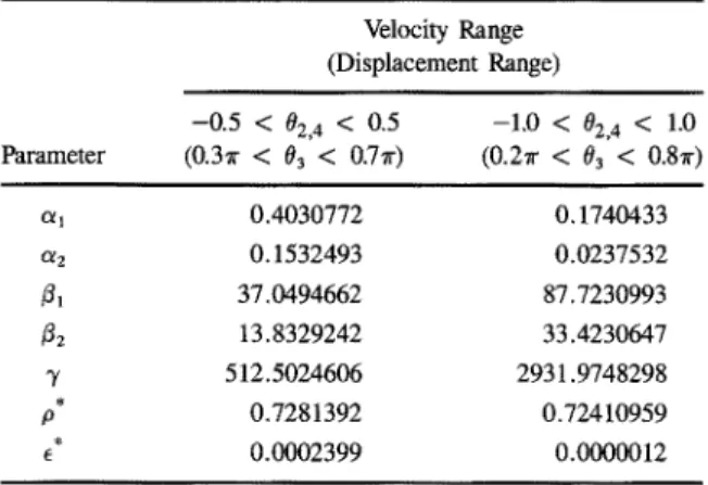
Table 1. Computed values of the parameters a¡, a2, fl¡, @2, y, p*
and e for two different regions.
Parameter « i « 2 0i 02 y p* e Velocity Range (Displacement Range) -0.5 < e2A < 0.5
(0.3ir < 03'< 0.7 TT)
0.4030772 0.1532493 37.0494662 13.8329242 512.5024606 0.7281392 0.0002399
-1.0 < e2A < 1.0
(0.2?r < 63' < 0.8ir)
0.1740433 0.0237532 87.7230993 33.4230647 2931.9748298 0.72410959 0.0000012
Table 2. Computed value of the parameter c for two different regions.
Velocity Range (Displacement Range)
-0.5 < e1A < o.5 - L O < e2A < i.o
Region ( 0 . 3 T < 03' < OJTT) (0.2TT < 93' < 0.8TT)
0.35T < 63R < 0.65ir 0.0014541 0.0097079
0.45x < 63R < 0.55x 0.0160932 0.0347817
For instance, suppose that the initial conditions 8¡ and initial estimate 0, satisfy v{0h fj¿)
< 0.0014541 and they are within the first region under study. The results provided in the tables imply that stability is preserved whenever the computer performs a logical time unit integration (or one iteration in the case of standard Newton technique) in less than 0.23 ms as determined by e*, and the tracking reference signal remains within — ir/4 < 0i#(i)
< u74 and 0.35ir < d3R(t) < 0.65s-. In the same way, for the second region of study for
which initial conditons 0¡ and initial estimate 0¡ satisfy v(6h $,) < 0.0347817 and the
track-ing signal is within - x / 4 < Qm{t) < x/4 and 0.45x < 03S(r) < 0.557T, stability is
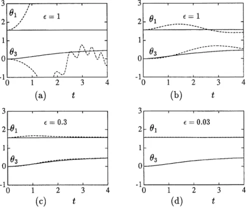
preserved when the computer performs a logical time unit integration in less than 1.2 /xs. Several simulations of the singularly perturbed system have been performed. It can be demonstrated that the above results are very conservative for this problem in which stability is guaranteed for a larger range of initial conditons and for larger values of e. Figures 6(a)-(d) present the time evolution of the joint displacements 0$) and 03(r) of the mechanical system
under study. The continuous lines represent an ideal evolution of the system in the case when the joint variables can be directly measured for control feedback. The reference point to be tracked is 0m = 0.5 and 03R = T/2 and the initial conditons chosen for the system
variables are 0¡ = 02 = 04 = 0 and 03 = ir/2. Figure 6(a) illustrates one case in which
initial guesses are chosen purposely to be 82 = fti = 0,6¡ = -?r/2, and §3 = —ir/2 to generate
1
. 0 1
Jh
3 1
I
e = l
2 -3 4 (b) Í -01
ii-0 1 1
e = 0.3
* 2 -i 3 4 1 0 -1
.0
1JL.
3 1
e = 0.03
-2 3 4
(c) t
(d)
Figure 6. Simulation of trajectories of example 2 for different values of e and initial guesses.
with the same value of the measurement vector x as the real mechanical system joint variables. In other words, x = A{ff) = A(6) but 9 & §. In this case, the inverse kinematics solver locates an undesired solution leading to pathological behavior. Note that, of course, the initial conditions and guesses do not satisfy sufficiency conditions obtained above to guarantee stability of the entire system. The rest of the figures correspond to initial guesses #2 = &i = 0 and §i = 03 = 0.5 and for different values of e. Note that the stability behavior
is good and it improves as e becomes smaller.
6. Concluding remarks
Some applications of the analysis of the dynamical system (1) to control theory have been developed. An updating control procedure has been proposed based on the iterative nature of the control algorithm. A singularly perturbed system formulation has been used to model both the combined dynamics of the system being controlled and a numerical iterative algo-rithm that is required to compute the control law. This approach can also be viewed as a combined controller and an observer (or an estimator) formulation. The results of Zufiria [1] regarding the behavior of a dynamical system that models these algorithms lead to a considerable simplification in the analysis. For the case of inverse kinematics control, it leads to a formulation in which the numerical algorithm that solves inverse kinematics can be considered as an observer (or an estimator) of the state variables. The study provides an estimate of the required speed of computations to preserve the stability of the chosen controller. In general such results are very conservative, and improvement is needed in that direction by obtaining less conservative bounds for the theorem based on the Lyapunov functions. The analysis carried out in this article can also be employed to compare different control laws and to select the one that provides less conservative results in the required speed of computation. Additional work is also needed for relaxing the assumption made in the modeling process. A combination of continuous-time and discrete systems (differential-difference equations) in a singularly perturbed structure, if possible, may lead to more accurate models.
Acknowledgments
The work reported here is partially supported by a grant from the National Science Foun-dation. Support from the USC Faculty Research and Innovation Fund is gratefully acknowledged. P.J. Zufiria also thanks the support of a Formación de Postgrado fellowship of the Programa Nacional de F.P.I, provided by the D.G.I.CT. of the Ministerio de Educación y Ciencia of Spain.
Notes
1. The computer algebra was performed by Macsyma.
References
1. P. J. Zufiria, Global Behavior of a Class of Nonlinear Dynamical Systems: Analytical, Computational and Control Aspects, Ph.D. dissertation, University of Southern California, 1989.
2. P.J. Zufiria and R.S. Guttalu, "On an application of dynamical system theory to determine all the zeros of a vector function," J. Math. Anal. Appl, vol. 152, 1990b pp. 269-295, 1990.
4. R.S. Guttalu and P.J. Zufiria, "On a class of nonstandard dynamical systems: singularity issues," in Adv. Cont. Dyna. Sys. vol. 34, (C.T. Leondes, ed.) pp. 279-324, Academic Press: New York, 1990.
5. R.C. Dorf, Modern Control Systems, Addison-Wesley: New \c-rk, 1986.
6. P. Kokotovic, H.K. Khalil, and J. O'Reilly, Singular Perturbation Methods in Control: Analysis and Design, Academic Press: London, 1986.
7. A. Saberi and H. Khalil, "Quadratic-type Lyapunov functions for singularly perturbed systems," IEEE Trans. AM. Cont., vol. AC-29, pp. 542-550, 1984.
8. L.T. Grugic, "Uniform asymptotic stability of non-linear singularly perturbed general and large-scale systems" Int. J. Cont., vol. 33, pp. 481-504, 1981.