Data driven control of DC DC power converters

Texto completo

(1)Instituto Tecnológico y de Estudios Superiores de Monterrey Campus Monterrey School of Engineering and Sciences. Data-Driven Control of DC-DC Power Converters A thesis presented by Benjamı́n Alejandro Frı́as Araya Submitted to the School of Engineering and Sciences in partial fulfillment of the requirements for the degree of Master of Science in Engineering Science. May 2019.

(2)

(3) Dedication (in Spanish) A mi familia, sin cuya ayuda esto simplemente no habrı́a sido posible. Hoy, este logro es mı́o gracias a ustedes..

(4) Acknowledgements (in Spanish) Agradezco a mi mamá, Mary Araya, por darme el conocimiento, apoyo y cariño necesarios para sobrevivir mis primeros dos años fuera de casa, y por atender mis llamadas diarias aunque fueran inoportunas y sin propósito. Por visitarme sinfı́n de veces y traerme un pedacito de casa cuando tanto lo añoraba. Gracias por todo, siempre. A mi papá, Benjamı́n Frı́as, por brindarme apoyo, sustento y cariño incondicional durante mis estudios de maestrı́a, y por enseñarme que la tenacidad, valor e intrepidez resuelven problemas mejor que cualquier otra fórmula. Gracias por todo, siempre. A mi hermana, Alejandra Frı́as, por enseñarme a poner mi propio bienestar mental sobre todas las cosas. Gracias por darme consejos y enviarme emojis para mitigar mi estrés. A mi asesor, Jonathan Mayo, por mostrarme que ser buena onda y un prodigio en el área de estudio no son caracterı́sticas mutuamente excluyentes. Por su paciencia y apoyo durante la elaboración de esta tesis, y por haber sembrado en mı́ una motivación por aprender. Trabajar contigo ha sido una experiencia increı́ble; gracias por transmitir tu conocimiento siendo siempre claro e interesado por el aprendizaje ajeno. A mi comité de tesis, Omar Ruiz y Servando López, por aceptar la tarea de revisar este trabajo. Su apoyo en implementaciones, observaciones e ideas fueron clave en el desarrollo y mejora de mi proyecto de tesis. A Luis y Ángel Bautista, por demostrarme que la amistad verdadera no conoce de fronteras. Por todas las horas de risas, videojuegos, discusiones y conversaciones desde lo más banales hasta lo más significativas. Luis, el Pı́pila no fue real. Ángel, ahı́ te hablo cuando me haya encantado la pelı́cula de Flight. Gracias a los dos por haber sido mis hermanos lejos de casa. Los llevo dentro siempre. A Enrique Soto, Angélica Orona, Marcela Herrera y Fabián Lugo, por haberme ayudado a mantener un equilibrio entre mi vida social y académica siendo excelentes amigos y personas. Espero CEDES no se sienta tan vacı́o sin mis visitas repentinas. Gracias por estar ahı́; los voy a extrañar mucho. A mis amigos tijuanenses por no hacerme extrañarlos tanto, y por ser la fuerza que a distancia me empujaba hacia delante. Nos vemos pronto; espero me reciban con tacos, pero de favor les suplico que tengan guacamole. Al Tecnológico de Monterrey por el apoyo otorgado con la beca de colegiatura, y a CONACYT por proveer manutención durante dos años. Este proyecto se llevó a cabo en tiempo y forma gracias, en gran parte, al sustento brindado por ambas organizaciones. Finalmente, a Griselda Ruiz por regalar su tiempo para escucharme. Gracias por contestar el teléfono ese dı́a..

(5) Data-Driven Control of DC-DC Power Converters by Benjamı́n Alejandro Frı́as Araya Abstract. In this thesis we develop a data-driven approach to the control design of power converters. We show that, given a set of measured data containing information about variables of interest (duty cycle as the input and inductor current/capacitor voltage as outputs) in the system, we can achieve asymptotic stability by solving a set of Lyapunov linear matrix inequalities (LMIs). This approach e↵ectively addresses the issue of performance degradation in controllers operating over networks, i.e. feeding constant power loads (CPL) as opposed to their standalone design, i.e. with nominal resistive loads. In order to do so, we study elements of behavioral system theory such as linear di↵erence systems and quadratic di↵erence forms; this allows for the creation of a framework compatible with higher-order discrete systems, which guarantees asymptotic stability in power converters both in standalone operation and with increased modeling complexity when interconnected to a network. Moreover, given the fact that the aforementioned LMIs provide us with multiple stabilizing gain solutions, we develop an algorithm for the synthesis of a switching multicontroller framework which, given a family of controllers, endeavors to select the single best-performing set in order to improve the dynamic profile of a to-be-controlled system, e.g. a power converter. Simulations and experimental results are provided as proof of concept, thus validating the theoretical material and illustrating the advantages of the proposed approaches..

(6)

(7) Contents Notation. ix. 1 Introduction 1.1 Overview of problem and contributions . . . . . . . . . . . . . . . . . . . . 1.2 Objective of the thesis . . . . . . . . . . . . . . . . . . . . . . . . . . . . . 1.3 Outline of the thesis . . . . . . . . . . . . . . . . . . . . . . . . . . . . . .. 1 2 5 5. 2 Continuous-time control of DC-DC converters 2.1 Preliminary background material . . . . . . . . . . . . . . 2.1.1 State space representations . . . . . . . . . . . . . 2.1.2 Lyapunov stability theory . . . . . . . . . . . . . . 2.2 Modeling of DC-DC power converters . . . . . . . . . . . 2.2.1 Large-signal modeling . . . . . . . . . . . . . . . . 2.2.2 Small-signal modeling: Approximate linearization . 2.3 Control of DC-DC power converters . . . . . . . . . . . . 2.3.1 Linear control design . . . . . . . . . . . . . . . . . 2.3.2 Commercial boost converter control: Gain tuning . 2.4 Multi-controller system . . . . . . . . . . . . . . . . . . . 2.5 Simulation Results . . . . . . . . . . . . . . . . . . . . . . 2.5.1 Open loop traditional boost converter . . . . . . . 2.5.2 Linear control of boost converter . . . . . . . . . . 2.5.3 Multi-controller switching system . . . . . . . . . . 2.6 Conclusion . . . . . . . . . . . . . . . . . . . . . . . . . .. . . . . . . . . . . . . . . .. . . . . . . . . . . . . . . .. . . . . . . . . . . . . . . .. . . . . . . . . . . . . . . .. . . . . . . . . . . . . . . .. . . . . . . . . . . . . . . .. . . . . . . . . . . . . . . .. . . . . . . . . . . . . . . .. . . . . . . . . . . . . . . .. 7 7 7 8 9 9 10 12 12 13 14 16 17 18 18 25. 3 Behavioral system theory 3.1 Linear di↵erence systems 3.2 Quadratic di↵erence forms 3.3 Lyapunov stability criteria 3.4 Conclusion . . . . . . . .. . . . .. . . . .. . . . .. . . . .. . . . .. . . . .. . . . .. . . . .. . . . .. . . . .. . . . .. . . . .. . . . .. . . . .. . . . .. . . . .. . . . .. 27 27 28 29 31. 4 Data-driven control of DC-DC converters 4.1 Data suitability: Hankel matrix criteria . . . 4.2 Classification of variables . . . . . . . . . . . 4.3 Persistency of excitation . . . . . . . . . . . . 4.4 Computation of coefficient matrices from data 4.5 Control design purely from data . . . . . . . 4.6 Gain computation . . . . . . . . . . . . . . . 4.7 Results . . . . . . . . . . . . . . . . . . . . . .. . . . . . . .. . . . . . . .. . . . . . . .. . . . . . . .. . . . . . . .. . . . . . . .. . . . . . . .. . . . . . . .. . . . . . . .. . . . . . . .. . . . . . . .. . . . . . . .. . . . . . . .. . . . . . . .. . . . . . . .. . . . . . . .. 33 33 34 34 35 37 39 40. . . . .. . . . .. . . . .. . . . .. . . . .. v. . . . .. . . . .. . . . .. . . . .. . . . ..

(8) vi. CONTENTS 4.7.1 4.7.2 4.7.3 4.7.4. Control of DC-DC converter with nominal resistive load . Control of DC-DC converter with DC machine load . . . Experiment: Control of DC-DC converter with constant load (CPL) . . . . . . . . . . . . . . . . . . . . . . . . . . Data-driven multi-controller system . . . . . . . . . . . .. . . . . . . . . power . . . . . . . .. . 40 . 44 . 46 . 50. 5 Conclusions and future work. 55. A MATLAB Codes A.1 Continuous-time . . . . . . . . . . . . . . . . . . . . . . . . . . . . . . . . A.1.1 Nonlinear model solver in open loop . . . . . . . . . . . . . . . . . A.1.2 Continuous-time control: Gain computation by Lyapunov LMI solving . . . . . . . . . . . . . . . . . . . . . . . . . . . . . . . . . . A.1.3 Nonlinear model solver in closed loop with multi-controller function A.2 Discrete-time . . . . . . . . . . . . . . . . . . . . . . . . . . . . . . . . . . A.2.1 Data extractor: Importing data from .txt file to MATLAB and reducing its integration step . . . . . . . . . . . . . . . . . . . . . . . A.2.2 Hankel matrix builder from data set in time-series form: Lag 1 . . A.2.3 Hankel matrix builder from data set in time-series form: Lag 2 . . A.2.4 Discrete-time control: Gain computation by Lyapunov LMI solving (LDS of lag 1) . . . . . . . . . . . . . . . . . . . . . . . . . . . A.2.5 Discrete-time control: Gain computation by Lyapunov LMI solving (LDS of lag 2) . . . . . . . . . . . . . . . . . . . . . . . . . . . A.2.6 Linearized model solver in closed loop . . . . . . . . . . . . . . . .. 59 59 59. Bibliography. 75. 61 62 67 67 68 69 70 71 73.

(9) List of Figures 1.1 1.2 1.3. Zooming on DC-DC converter operating over a network for control purposes. . . Controller re-design process via data-driven approach. . . . . . . . . . . . . . . General diagram of switching control [1]. . . . . . . . . . . . . . . . . . . . . .. 2.1 2.2 2.3 2.4 2.5 2.6 2.7 2.8 2.9 2.10 2.11 2.12 2.13 2.14 2.15 2.16 2.17 2.18. Traditional boost converter topology. . . . . . . . . . . . . . . . . . . . . Topologies induced by switching. . . . . . . . . . . . . . . . . . . . . . . General feedback controller for a linearized converter. . . . . . . . . . . . Predefined feedback controller example. . . . . . . . . . . . . . . . . . . Multi-controller operation. . . . . . . . . . . . . . . . . . . . . . . . . . Boost converter simulation results. . . . . . . . . . . . . . . . . . . . . . Controlled boost converter simulation results. . . . . . . . . . . . . . . . Algorithm for controller bank generation. . . . . . . . . . . . . . . . . . Stabilizing controller bank for n = 40. . . . . . . . . . . . . . . . . . . . Multi-controller structure performance for ✏ = 0.1. . . . . . . . . . . . . . Multi-controller structure performance for ✏ = 0.01 and di↵erent trajectory. Multi-controller structure performance for varying ✏ (0.3). . . . . . . . . . Multi-controller structure performance for varying ✏ (0.2). . . . . . . . . . Multi-controller structure performance for varying ✏ (0.01). . . . . . . . . Multi-controller performance under abrupt changes in output resistance. . Multi-controller performance under abrupt changes in input voltage. . . . Multi-controller performance for trajectory following. . . . . . . . . . . . Changes in controller set index i for multi-controller system. . . . . . . . .. . . . . . . . . . . . . . . . . . .. 9 9 12 13 16 17 19 19 20 21 22 22 23 23 24 24 25 25. 4.1 4.2 4.3 4.4 4.5 4.6 4.7 4.8 4.9 4.10 4.11 4.12 4.13 4.14 4.15. e from measurement data. Algorithm for the computation of the coefficient matrix R General realization of a data-driven feedback controller in state space form. . . . Predefined feedback controller example. . . . . . . . . . . . . . . . . . . . . . Varying input signal. . . . . . . . . . . . . . . . . . . . . . . . . . . . . . . . Boost converter with variable input used to gather data. . . . . . . . . . . . . . Unstable voltage response for data gathering. . . . . . . . . . . . . . . . . . . Control circuit implemented in PSIM. . . . . . . . . . . . . . . . . . . . . . . . Circuit response to data-driven controller. . . . . . . . . . . . . . . . . . . . . Disturbance rejection at time step t = 0.4s. . . . . . . . . . . . . . . . . . . . Boost converter with DC machine load. . . . . . . . . . . . . . . . . . . . . . Unstable voltage response for data gathering in DC machine-loaded circuit. . . . Controlled voltage of a Boost converter with DC machine load. . . . . . . . . . Controlled current in Boost converter. . . . . . . . . . . . . . . . . . . . . . . Source and load converters and corresponding controllers. . . . . . . . . . . . . Experimental setup. . . . . . . . . . . . . . . . . . . . . . . . . . . . . . . .. 36 38 39 41 41 42 43 43 43 44 45 45 46 47 48. vii. . . . . . . . . . . . . . . . . . .. . . . . . . . . . . . . . . . . . .. 3 4 5.

(10) viii. LIST OF FIGURES 4.16 Input current iin and output voltage vC1 behavior under abrupt changes at the input voltage vin . . . . . . . . . . . . . . . . . . . . . . . . . . . . . . . . . 4.17 Instability in the source converter produced by the connection of a constant power load. . . . . . . . . . . . . . . . . . . . . . . . . . . . . . . . . . . . 4.18 Source converter’s input current i and output voltage v stabilization derived from modifying the control strategy. . . . . . . . . . . . . . . . . . . . . . . 4.19 Discrete-time algorithm for controller bank generation. . . . . . . . . . . . . 4.20 Stabilizing controller bank for n = 40. . . . . . . . . . . . . . . . . . . . . . 4.21 Multi-controller strategy implemented in PSIM. . . . . . . . . . . . . . . . . 4.22 Output behavior with (a) a single controller, (b) the multi-controller strategy. .. . 49 . 49 . . . . .. 50 51 52 53 53.

(11) Notation Iq AT col(A, B). Identity matrix of dimension q ⇥ q. Transpose of matrix A.. If A and B are matrices with the same number of columns, it denotes the matrix obtained by stacking A over B.. R. Set of real numbers.. Z. Set of integers.. Z+. Set of positive integers.. Rq. Space of real vectors of dimension q.. Rp⇥q. Space of p ⇥ q dimensional real matrices.. R•⇥•. Space of real matrices with an unspecified number of rows and columns.. rank(A) colspan(A). Rank of a given matrix A 2 R•⇥• .. Column span of A, i.e. the set of all possible linear. combinations of its column vectors. ( f )(t). Shift operator applied to a function f : Z+ ! Rq .. Defined as ( f )(t) := f (t + 1), and can be of order N in general, i.e. (. N f )(t). ix. := f (t + N )..

(12)

(13) Chapter 1. Introduction In recent years, renewable energy research has been deemed as one of the key points to leading the planet into a more sustainable framework. The main motivation behind the growing use of renewables is to reduce dependence on fossil fuels and greenhouse gas emissions. Power converters have thus been a core element of such research, since their usefulness lies in their ability to overcome some of the inherent limitations imposed by the use of renewable energy sources (e.g. low voltage outputs, intermittency caused by environmental conditions, difficulty of interconnection with other sources). As such, multiple strategies for robust control of power converters have been successfully implemented (see e.g. [2–4]). However, a great number of these control schemes are tested on converters designed for stand-alone operation, i.e. considering a nominal resistive load connected at the output. Therefore, when these converters are connected to an integrated system, e.g. an energy distribution network, the interaction between subsystems may cause significant performance degradation, or – in the worst-case scenario – instability due to the negative impedance inherent to regulated power devices such as constant power loads (CPLs). In order to mitigate such issues, we usually employ model-based paradigms; we assume that a model representing the full DC network is readily available for us to design stabilizing control strategies. Examples of such model-based approaches include: [2–4], where control structures are implemented in order to regulate boost converters feeding CPLs; [5–9], where the asymptotic stability of cascaded DC-DC converters is studied; [10–13], where e↵orts are made to mitigate the e↵ect caused by negative impedance in a load converter, therefore inducing stability; [14–16], where new stabilization methods, such as damping enhancement and sliding mode control for CPL-loaded controllers, are introduced.. 1.

(14) 2. Chapter 1 Introduction. Evidently, these contributions center their theoretical development on the availability of a full network model, particularly in state space form, i.e. using sets of first order di↵erential equations. It is well-known that there exists a high amount of available mathematical tools and environments compatible with state space representations. Moreover, the study of stability properties for such systems can be easily carried out by means of linear matrix inequalities (LMIs). Following these ideas, the fact that such is the mainly used modeling approach is a natural consequence. Higher-order representations, on the other hand, are traditionally dropped in favor of first-order systems due to a shortage of mathematical and computational tools available for studying their dynamics and stability. [17] However, state space models of networks are not a given [17], and in some cases their derivation is in a higher level of complexity, especially when introducing a higher number of state variables to the model or when considering the practical scenario of parasitic elements with energy storage or time delay properties; their presence in a circuit causes the addition of at least one more state variable or di↵erential equation to the model. This challenge is recognized by researchers in the field of smart grids [18], who argue that traditional modeling techniques may not be entirely useful in studying scenarios where the complexity of networks becomes increasingly higher. Prompted by these challenges, new model-less control techniques have surfaced in order to overcome the aforementioned modeling shortcomings. These techniques involve datadriven approaches that guarantee stability in a deterministic way, without the need for mathematical models. For example, [19] proposes data-driven control structures for interconnected microgrids by using measurement data and state observers. In [20], a generic model recreation for a microgrid is proposed by considering input/output measurement data. The aforementioned solutions succeed in providing novel model-less approaches to stability; however, in most cases the technique requires either an identification of pre-defined mathematical models, or a high number of sensors due to the increasing number of state variables. Therefore, they do not consider the possibility of representing the full network dynamics and –a common occurrence in practice– with a limited number of sensors. Motivated by these issues, in this thesis we present a data-driven deterministic approach to stability of power converters.. 1.1. Overview of problem and contributions. It is known that a power converter tested in standalone design can be robustly regulated at a desired equilibrium point. However, as previously discussed, when the converter operates over a network, interconnections between subsystems cause a capacitor current.

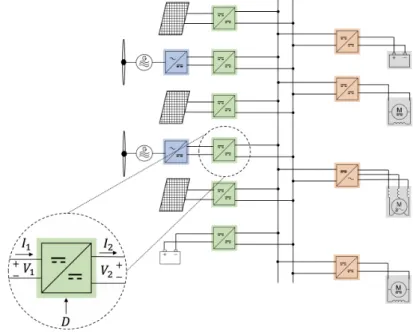
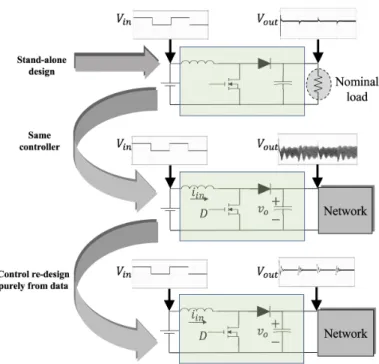
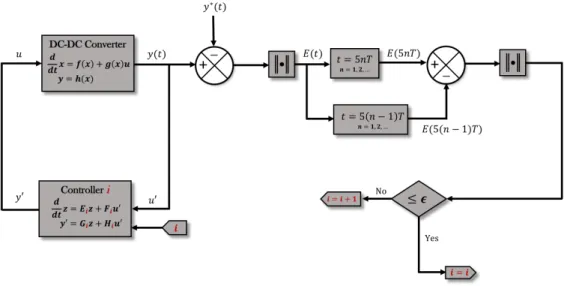
(15) Chapter 1 Introduction. 3. imbalance which destabilizes the previously stable capacitor voltage, thus steering the output into an undesirable behavior. In order to mitigate this issue, our main contribution is to propose a framework where we adopt a general view of a network as a group of interconnected subsystems interacting with each other via electrical and control variables (currents, voltages and duty cycles respectively). Therefore, in order to design stabilizing controllers, we zoom into the network and focus on the to-be-controlled converter. This process is shown in Fig. 1.1.. Figure 1.1: Zooming on DC-DC converter operating over a network for control purposes.. After zooming into a specific converter, we determine the variables of interest through which the subsystem interacts with the network. We then apply a system identification algorithm based on measured data from such converter variables, and use discrete-time Lyapunov theory in order to determine stabilizing controllers via solutions of a discretetime LMI. Such a procedure allows for a mathematically rigorous re-designing of controllers whenever their behavior becomes unstable by network interconnections, i.e. in the CPL problem shown in [6, 21–24]. This strategy is depicted in Fig. 1.2. As a secondary contribution, we benefit from the fact that solving the Lyapunov LMI in multiple instances during control design allows for the existence of multiple controller gain sets. These gain sets can be stored in a controller bank and used in the development of a switching controller framework. As discussed in [1], the use switching control systems is motivated by a problem arising when, given a process typically described by a continuous-time control system, we need to find a controller such that the closed-loop system displays a desired behavior. In some cases, this feedback controller may not exist. In such situations, a possible alternative is to incorporate logic-based decisions into the control law and implement switching among.

(16) 4. Chapter 1 Introduction. Figure 1.2: Controller re-design process via data-driven approach.. a family of controllers. Thus, a hybrid closed-loop system is generated, which is able to induce di↵erent sets of continuous-time dynamics based on discrete switching actions. Consider, for example, the case of nonholonomic systems described in [1]; such systems are subject to constraints involving both the state and its derivative. Therefore, they cannot be asymptotically stabilized by a continuous feedback controller. We can single out the following motivating points in control problems for which we would need to consider switching control: • In many realistic scenarios, continuous control is not suitable; i.e., there exist a set of desired dynamics which are not achievable by means of continuous control.. • The system model is highly uncertain, and a single continuous control law cannot be found.. • If a given process is prone to unpredictable external influences or component fail-. ures, then it may be necessary to consider discontinuous control as a way to ensure adaptability and robustness in the control scheme.. Based on these ideas, in this thesis we also present a switching, adaptable multi-controller strategy and test it on boost converters. Particularly, the family of controllers is generated by solving the Lyapunov stability problem in multiple instances, and the logic by which the controller switches into each possible scenario is given by an arbitrarily imposed switching condition, i.e. a logical decision-making step; this ensures adaptability in the control process. This is depicted schematically in Fig. 1.3..

(17) Chapter 1 Introduction. 5. Figure 1.3: General diagram of switching control [1].. 1.2. Objective of the thesis. Following the aforementioned ideas, the specific research objectives to which we contribute with this thesis are listed below: • To develop a data-driven control strategy for DC-DC power converters (both in. standalone and interconnected operations) which bypasses the need for mathematical models and guarantees asymptotic stability.. • To introduce a switching multi-controller framework which steers the plant output dynamics as close as possible to an unknown, desired trajectory.. 1.3. Outline of the thesis. We now describe the contents of this thesis. • Chapter 2. We review fundamental concepts related to average modeling, lin-. earization and control of DC-DC power converters. We also introduce the notion of Lyapunov stability conditions as a mathematical tool for stabilizing gain computation. Finally, we propose new results regarding a switching multi-controller structure. In this chapter, theoretical material is verified with MATLAB simulations.. • Chapter 3. We begin the study of discrete time systems, introducing higher-. order representations in linear di↵erence systems (LDS). Moreover, we establish quadratic di↵erence forms (QdFs) as a means of studying stability properties of a LDS. Moreover, further analysis regarding Lyapunov stability theory is given and a discrete-time version of the conditions in Chapter 2 is developed.. • Chapter 4. We propose an approach to data-driven control of DC-DC converters.. We introduce the notion of data-based matrices, and establish necessary conditions for a set of measured data to be sufficiently informative about the system dynamics.

(18) 6. Chapter 1 Introduction in order to recreate its model. With this recreated model, we develop an algorithm to stabilize converters both in standalone operation and when connected over networks. We also present results regarding a proposed switching multi-controller structure which uses data-driven controllers. In this chapter, theoretical material is verified by means of PSIM simulations and experimental validation. • Chapter 5. We provide general conclusions and establish future research directions for the hereby presented work.. Appendix A contains all the MATLAB codes written for testing the theoretical material hereby developed..

(19) Chapter 2. Continuous-time control of DC-DC converters In this chapter we introduce general concepts of continuous-time power converter modeling and control. We focus our study on the boost converter and develop a control strategy using Lyapunov criteria; such an analysis is instrumental for building a framework around the key content of this thesis. Finally, we present a switching multi-controller algorithm which uses the same Lyapunov-based approach to guarantee plant stability under specific performance conditions.. 2.1. Preliminary background material. For ease of reference and in order to make this work self-contained, we first introduce some fundamental theoretical material which will be continuously referred to for the remainder of this chapter.. 2.1.1. State space representations. As discussed in [25], a state space representation for any linear, time-invariant system has the general form d x = Ax + Bu ; dt y = Cx + Du ;. (2.1). where x : R ! Rn is the state vector comprised of n state variables, u : R ! Rm is the input vector comprised of m input variables, while A 2 Rn⇥n , B 2 Rn⇥m , C 2 Rp⇥n. and D 2 Rp⇥m are coefficient matrices. Finally, y : R ! Rp is referred to as the output vector.. 7.

(20) 8. Chapter 2 Continuous-time control of DC-DC converters. Now consider the case where the input u is state-dependent, e.g. u = By letting C = 0 and D = 0, then substituting u in (2.1), we obtain:. kx with k 2 Rn .. d x = Âx ; dt where Â = (A. (2.2). Bk) 2 Rn⇥n is a new coefficient matrix. Due to the lack of an input. in its model, (2.2) is commonly referred to as an autonomous system. In the following,. we show how in state-space modeling, studying system stability requires a system to be autonomous.. 2.1.2. Lyapunov stability theory. When controlling a given dynamical system, we are interested in studying its behavior in terms of stability. Thus, we first introduce a classic definition [26], i.e. a linear system represented by (2.2) is asymptotically stable if limt!1 x(t) = 0 for all x that satisfies (2.2). This definition allows for a general understanding of the implications behind stable system behavior. However, for control design purposes, it becomes necessary to study such a concept in terms of mathematical specifications. Therefore, we now introduce the notion of Lyapunov criteria: Theorem 2.1. [26] A system represented by (2.2) is asymptotically stable if there exists a state function V (x) such that, for all x that satisfies (2.2), it holds that: 1) V (x) and 2). d dt V. 0,. (x) < 0. Thus, V (x) is called a Lyapunov function for (2.2).. Consider the autonomous system described by (2.2), and let the candidate function for Theorem 2.1 be the quadratic state function V (x) = xT P x, where P = P T > 0 is an unknown matrix. Taking the time derivative of the state function by means of the chain rule yields: d d d V (x) = xT P x + xT P x dt dt dt T T T = x Â P x + x P Âx. (2.3). = xT (ÂT P + P Â)x . Thus, in order for Theorem 2.1 to hold, it must follow that ÂT P + P Â < 0 .. (2.4). Notice that (2.4) is known as a linear matrix inequality (LMI). Therefore, given any linear system, its stability can be verified by numerically computing a matrix P which satisfies (2.4). This can be done by means of standard LMI solvers, such as Yalmip [27]. Such a toolbox consists of an add-on to the numerical environment MATLAB, and.

(21) Chapter 2 Continuous-time control of DC-DC converters. 9. is used to solve feasibility problems related to linear inequalities with a specified set of constraints. We have given a brief introduction to state-space representations and stability for dynamical models; in the following, we show how to obtain such models from DC-DC power converters.. 2.2. Modeling of DC-DC power converters. We now discuss a procedure for determining mathematical models describing power converter dynamics in a rigorous manner. We first focus on large-signal modeling in order to describe such converters in terms of the underlying nonlinear equations. Then we study small-signal modeling, which approximates the large-signal behavior with linear equations. Note that the latter is particularly useful when attempting control design on power converters.. 2.2.1. Large-signal modeling. Let us consider the traditional boost converter with a nominal resistive load, as depicted in Fig. 2.1.. Figure 2.1: Traditional boost converter topology.. The values of the discrete switching variable u 2 {0, 1} induces two possible circuit. topologies, as illustrated in Fig. 2.2. Thus, we can obtain their dynamics by applying Kirchho↵s laws in each case.. Figure 2.2: Topologies induced by switching.. Consider the circuit in Fig. 2.2 a. When the switching variable is set to u = 1 , Kirchho↵’s voltage and current laws yield the following dynamics:.

(22) 10. Chapter 2 Continuous-time control of DC-DC converters 8 d > > < L i = vin dt > > :C d v = v dt R. (2.5). Conversely, let us now consider the circuit in Fig. 2.2 b. When the switching variable is set to u = 0 , Kirchho↵’s voltage and current laws yield the following dynamics: 8 d > > < L i = v + vin , dt > > :C d v = i v . dt R. (2.6). By comparing both sets of equations and introducing the switching variable u as a parameter, we obtain a unified dynamic model for the circuit, described by: 8 d > > < L i = (1 u)v + vin , dt > > : C d v = (1 u)i v . dt R. (2.7). Equation set (2.7) represents the switched model of the boost converter. This representation emphasizes the discrete nature of the input variable u. However, when working with periodic switching signals, it becomes necessary to consider the average value of the input variable over a switching time period [28]. Therefore, the previously discrete switching variable u now becomes a continuous average switching variable, i.e. d 2 [0, 1] . We refer to d as the duty cycle.. Finally, we obtain the average model of the boost converter by replacing the discrete switching variable in the switched model (2.7) with its continuous equivalent: the duty cycle. Thus, the average model is given by 8 d (1 d) vin > > v+ , < i= dt L L > 1 > : d v = (1 d) i v. dt C RC. (2.8). Notice that multiplication between variables makes such a model nonlinear. Remark 2.2. In equation sets (2.5 - 2.7), state variables [i v] are defined as instantaneous. However, when used in (2.8) –and for the rest of this thesis–, such variables are reformulated in average terms.. 2.2.2. Small-signal modeling: Approximate linearization. Through a linearization process, nonlinear models can be approximated –around a specific point– by a linear equivalent. However, this new model is only valid in a region near.

(23) Chapter 2 Continuous-time control of DC-DC converters. 11. the selected point. As discussed in [28], in nonlinear DC-DC power converters, approximate linearization-based feedback controllers usually perform stabilization to a desired equilibrium value even when the dynamics of the controlled converter start at the origin, i.e. when the initial conditions of such a system are far away from such an equilibrium. This optimal performance can be attributed to the fact that DC-DC power converters have one single equilibrium point for each input/output variable, unlike highly nonlinear systems which could possibly have a larger number of equilibria (e.g. Furuta pendulum). Based on these ideas, we derive a linearized model in order to design a controller for a nonlinear boost converter. Let u : R ! Rm and y : R ! Rn be the input/output variables available in a system. In a boost converter, the input u := d is the duty cycle, and the output y := col(i, v). contains the input current and output voltage. Thus, let w := col(u, y) be the global set of variables of interest in a boost converter. Consider the boost converter model described by (2.8). We can begin to linearize this model about an arbitrary equilibrium point by defining error variables for each input/output in the nonlinear system, i.e. ŵ := w. w̄ ;. where w̄ contains the values of the variable set at the fixed equilibrium. The following analogous notation for the input-output partition is used: ŵ = col(û, ŷ) . Finally, we can complete the linearization process by performing a Taylor series expansion of (2.8). For ease of reference, we recall the theoretical details behind such a concept. Consider a dynamical system described in general by d yk = fk (y1 , y2 , . . . yn , u1 , u2 , . . . um ), k = 1, 2, . . . n , dt with error variables ŷ and û. A Taylor series expansion of fk about the equilibrium points such that fk (y¯1 , y¯2 , . . . y¯n , u¯1 , u¯2 , . . . u¯m ) = 0, is given by 0 1 n m X X d @fk @fk A ŷk = @ yˆj + uˆj dt @yj @uj j=1. j=1. (2.9) y=y u=u. Now consider the nonlinear boost converter model in (2.8). As per (2.9), we can linearize ¯ Taking partial derivatives and evaluating at the this model about equilibria ī, v̄, d. corresponding equilibria yields the linearized model of the boost converter, given by:.

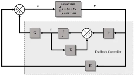
(24) 12. Chapter 2 Continuous-time control of DC-DC converters 8 ¯ d (1 d) v̄ > > v̂ + dˆ , < î = dt L L > ¯ > 1 ī ˆ : d v̂ = (1 d) î v̂ d. dt C RC C. 2.3. (2.10). Control of DC-DC power converters. We now use the aforementioned linearized converter model in order to generate linear feedback controllers which, when interconnected with a nonlinear converter model, guarantee asymptotic stability by means of Lyapunov criteria.. 2.3.1. Linear control design. In this analysis we do not impose a particular controller structure (proportional (P), proportional-integral (PI), proportional-integral-derivative (PID)), but instead we adopt a general point of view for control design and let the specific application dictate the type of controller to be used. Therefore, a feedback controller can adopt a general form 8 < d z = Ez + F u0 , dt : y 0 = Gz + Hu0 ;. (2.11). where z : R ! Rp , E 2 Rp⇥p , F 2 Rp⇥n , G 2 Rm⇥p , H 2 Rm⇥n . In order to perform. an interconnection between such a controller and a linear plant e.g. (2.1), let us define the controller input/output variables as u0 := y and y 0 := u, respectively. This process is depicted in Fig. 2.3.. Figure 2.3: General feedback controller for a linearized converter.. Note that this general family of controllers admits any P, PI, PID, state- and outputfeedback configurations, among many other suitable possibilities..

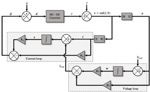
(25) Chapter 2 Continuous-time control of DC-DC converters. 13. Let us now consider the linear plant in (2.1), as well as the controller in (2.11). By redefining the controller variables as shown in Fig. 2.3, we obtain the complete set of equations describing the plant-controller combination: 8 d > x = Ax + Bu ; > > > < dt d z = Ez + F x ; > > dt > > : u = Gz + Hx .. (2.12). By straightforward algebraic manipulation of (2.12), the general plant-controller combination can thus be represented as: " # " #" # A + BH BG x d x = . dt z E F z. 2.3.2. (2.13). Commercial boost converter control: Gain tuning. The general plant-controller structure in (2.12) allows us to proceed without imposing a particular control scheme, but instead letting the specific application be the determining factor for such a decision. Let us consider the particular case of a commercial boost converter whose manufacturer’s pre-defined controller only allows for gain modification and consists of a double loop current-voltage nested controller, as depicted in Fig. 2.4.. Figure 2.4: Predefined feedback controller example.. We observe that such a controller consists of the following equations: 8 < d w = v̂ v̂ref , dt Voltage loop: : îref = g1 w g2 v̂ ;. (2.14).

(26) 14. Chapter 2 Continuous-time control of DC-DC converters 8 < d z = î îref , dt Current loop: : ˆ d = k1 z k2 î ;. (2.15). where w, z : Z+ ! R and ki , gi , i = 1, 2, are scalar quantities known as gains. Given this set of equations and considering the general state space model for linearized converters d x = Ax + Bu , dt ˆ we can construct the converterby recalling that x := col(î, v̂) and letting u := d, controller combined model: 2 3 2 x A k2 B[1 0] d 6 7 6 4 z 5 = 4[1 0] + g2 [0 1] dt w [0 1] | {z } | {z d 0 x dt. k1 0 0. Â. 32 3 x 76 7 g1 5 4 z 5 . 0 w } | {z }. 02⇥1. (2.16). x0. Controller gains ki , gi , i = 1, 2, which guarantee converter stability, can thus be computed using (2.4). Since in this case parameters from both Â and P are unknown, condition (2.4) is a bilinear matrix inequality whose solutions can be computed using standard LMI solvers such as Yalmip.. 2.4. Multi-controller system. As discussed in Chapter 1, a special category of hybrid systems known as switched systems, considers continuous-time systems coupled with discrete switching events. Thus, we will now focus on the development of a switched multi-controller operation for a controlled converter such as the one described by (2.16). In order to further understand the proposed multi-controller framework, we briefly recall the motivation behind its development. In Chapter 1, we argue that discontinuous control schemes allow for achievements in dynamics which are not possible using purely continuous feedback. Moreover, due to the logic-based part of its operation, switching control brings a sense of adaptability to the overall scenario. In terms of power converters, discontinuous feedback allows for a more robust variable (e.g. voltage) regulation despite abrupt changes in the load, in comparison to continuous control methods which may not respond as adequately. Moreover, a multi-controller framework is also useful in cases where we become interested in trajectory tracking for any purpose; notable examples of such a situation are techniques such as maximum power point tracking [29] and enveloped tracking[30]. Constant voltage regulation –a common objective in power converter control– is not the main purpose in.

(27) Chapter 2 Continuous-time control of DC-DC converters. 15. these cases; they instead focus on following specific trajectory. For such purpose, an adaptable discontinuous controller is a plausible solution. Following the above ideas, the concept of switching control can applied to a controlled boost converter as in (2.16) by noticing that the stability condition in (2.4) is an inequality, i.e. it allows for multiple solutions. Therefore, by solving such an inequality and thus performing gain computation in multiple instances, we generate a “bank” or “family” of admissible (i.e. stabilizing) controller gains which will guarantee asymptotic stability when applied to the boost converter. Having multiple gain sets implies the existence of various possible control scenarios (one for each gain set); these scenarios can be switched into depending on a state-related condition. Evidently, each of these control scenarios will steer the plant into a new set of asymptotically stable dynamics. We now introduce the preliminaries for the switching condition. Let the instantaneous error E(t) be defined as: E(t) =| y(t). y ⇤ (t) | ,. (2.17). where: • y(t) is the instantaneous converter output (e.g. output voltage); • y ⇤ (t) is a desired trajectory. We therefore establish the switching condition for the multi-controller system as: | E(5nT ). E(5(n. 1)T ) | ✏ ,. (2.18). where: • n = 1, 2, . . . is a scalar quantity measuring time steps; • T denotes the integration step for the numerical method used to solve the dynamical model;. • ✏ is a scalar quantity known as performance condition for the multi-controller system, and is associated to the maximum allowed error rate between the real and desired dynamics. As depicted in Fig. 2.5, condition (2.18) is used to induce switching between di↵erent controller gain sets based on the di↵erence between the real output and an arbitrary desired trajectory. This instantaneous error is compared every 5 time steps and is.

(28) 16. Chapter 2 Continuous-time control of DC-DC converters. equivalent to measuring the derivative of the error variable. If such a derivative exceeds an admissible value ✏, the system will switch into a di↵erent set of controller gains in an attempt to reduce future propagation of the error. In other words, the goal of this switched system is to steer the output “as close as possible” to an arbitrary desired behavior, by switching between controller gain sets when the rate of change of the error becomes unacceptable for the expected performance conditions.. Figure 2.5: Multi-controller operation.. Remark 2.3. In this work we ponder the following classic considerations for switching multi-controller systems: • To ensure stability, multiple plant-controller combined systems could share a common Lyapunov function.. • To ensure stability, multiple plant-controller combined systems could have a multiple Lyapunov function.. • Between switching instants, a certain dwell time must be considered in order for. the system to approximate the equilibrium as much as possible; this prevents instability. In this work, we consider the dwell time to be 5nT .. However, since these points are not part of the main scope of this thesis, we refer the reader to [31] for more details.. 2.5. Simulation Results. Simulations were carried out in order to verify the theoretical material discussed above. In the case of continuous-time systems, we use the standard numerical environment MATLAB to test the validity of every concept described in this chapter..

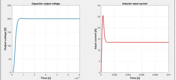
(29) Chapter 2 Continuous-time control of DC-DC converters. 2.5.1. 17. Open loop traditional boost converter. As previously discussed and given the focus of this chapter, we first simulate a traditional boost converter in open-loop configuration as depicted in Fig. 2.1, with the nominal parameters shown in Table 2.1. Table 2.1: Nominal parameters for simulation.. Notation. Parameter description. Value. Vin. Input voltage. 30V. V̄. Output voltage at equilibrium. 200V. L. Inductor. 250µH. C. Capacitor. 10µF. R. Load resistance. 100⌦. h. Time step for numerical method. 1µs. We carry out this simulation using the average model described by equation set (2.8). Using such equations, we can easily verify that the equilibrium values for duty cycle and current must equal v̄ d¯ =. vin v̄. = 0.85 ;. v̄ ī = R. ✓. 1 1. ◆. = 13.333 A . d¯. (2.19). We use the Forward-Euler numerical method to perform the simulation, solving the boost converter model described by (2.8). Simulation results are shown in Fig. 2.6.. Figure 2.6: Boost converter simulation results.. Notice that the equilibrium values of both the voltage and the current in the simulation are as expected..

(30) 18. Chapter 2 Continuous-time control of DC-DC converters. For a detailed description of the MATLAB codes written for simulation purposes, please refer to Appendix A.. 2.5.2. Linear control of boost converter. We carry out a second simulation, now centered on solving the combined convertercontroller model described by equation (2.16). The motivation behind this simulation is to test the validity of the ideas discussed in section 2.2.2, in which we argue that linear feedback controllers perform adequately when applied to nonlinear plants with a single equilibrium point, e.g. power converters. To this purpose, consider the same boost converter as in Subsection 2.5.1, with nominal parameters described in Table 2.1 and equilibrium values defined in (2.19). From its linearized version described by (2.10), let the state space representation matrices A :=. ". 0 ¯ (1 d) C. ¯# (1 d) L 1 RC. ;. B :=. ". v̄ L ī C. #. .. Such matrices can thus be used in the combined model described by (2.16). Moreover, using such a model’s coefficient matrix, we solve the Lyapunov inequality (2.4) in order to compute stabilizing controller gains. Such a process yields the gain set k1 := 0.0047 ;. k2 := 0.0141 ;. g1 := 16.8823 ;. g2 := 10.9711 .. By recalling that these gains come from a linear model, we now use them in order to control the nonlinear system described by (2.8). To this purpose, we let the input d := dˆ+ d¯ and once again solve the nonlinear converter model by means of the ForwardEuler numerical method. Evidently, the value of d will vary with each iteration in order to satisfy the conditions of the control structure in (2.15). The results of this simulation are shown in Fig. 2.7. Notice that aside from maintaining the voltage and current at the desired equilibrium points, the established control structure causes a relevant improvement in signal quality (particularly noticeable in the output voltage waveform) where the transient’s overshoot, oscillation and response time are significantly reduced.. 2.5.3. Multi-controller switching system. In Subsection 2.5.2 we focused on controlling a boost converter using Lyapunov stability criteria. We now extend this idea to a proof of concept regarding the multi-controller system discussed in section 2.4, where the inequality (2.4) is solved in multiple instances.

(31) Chapter 2 Continuous-time control of DC-DC converters. 19. Figure 2.7: Controlled boost converter simulation results.. Figure 2.8: Algorithm for controller bank generation.. in order to generate a “bank” of admissible, stabilizing controllers for the converter. The general algorithm for this process is shown in Fig. 2.8. The algorithm consists of a linearization of the bilinear matrix inequality (2.4); we achieve this by starting the algorithm with gain values (embedded in matrix Â) which are very close to 0, thus reducing the number of unknown parameters to one, i.e. matrix P , and e↵ectively transforming the Lyapunov condition into a linear matrix inequality (LMI). After computing P , we use it as a known parameter to compute a new, unknown gain set. We then use such a gain set as a known parameter to compute a new P matrix. We refer to this process as a linearizing loop, which is repeated to generate n controller gain sets. Note that all n gain sets guarantee asymptotic stability, given that they are generated under Lyapunov criteria..

(32) 20. Chapter 2 Continuous-time control of DC-DC converters. The process of computing multiple stabilizing gain sets leads to the generation of a gain matrix defined as 2. k 11. 6 6 k 12 Cn := 6 6 .. 4 .. k 1n. k 21. g 11. k 22 .. .. g 12 .. .. k 2n. g 1n. g 21. 3. 7 g 22 7 .. 7 7 ; . 5. g 2n. whose n number of rows are comprised of the gain sets computed using the algorithm in Fig. 2.8. Such an algorithm was used to compute multiple stabilizing gains for the same boost converter used in previous subsections (refer to Table 2.1 and (2.19) for parameters). Starting the algorithm with initial conditions k1 := 0.001 ;. k2 := 0.0001 ;. g1 := 0.0001 ;. g2 := 0.0001 ,. we apply the algorithm in Fig. 2.8 by means of the Yalmip solver. For n = 40, Fig. 2.9 shows the gain matrix C40 in table form.. Figure 2.9: Stabilizing controller bank for n = 40.. Notice that even though the algorithm starts at values which are practically zero, the values of ki , gi , i = 1, 2 exhibit linear convergence to an unknown value as we repeatedly solve the gain computation algorithm. Even though the final value of convergence is uncertain, we do not focus on unraveling it; rather, we take advantage of the fact that this convergence process provides us with various controller gains which guarantee asymptotic stability for the boost converter..

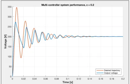
(33) Chapter 2 Continuous-time control of DC-DC converters. 21. As discussed in section 2.4, having multiple controller gains implies the possibility of creating a control system which switches into each gain set according to a certain performance condition; we simulate such an idea as a proof of concept using the same boost converter as in previous subsections. Consider the controlled boost converter in section 2.5.2. Using MATLAB, we extend such a simulation to include the multi-controller system; namely, we consider the gain matrix C40 shown in Fig. 2.9 as well as condition (2.18) for automatic switching into each gain set. We establish the desired trajectory to be y ⇤ (t) = 200[1. e. 290t. cos (700t)] ,. as well as a maximum allowed error rate of ✏ = 0.1. Results of this simulation are shown in Fig. 2.10. Notice that, as expected by design, the multi-controller system steers the output as close to the desired trajectory as possible within the allowed error rate.. Figure 2.10: Multi-controller structure performance for ✏ = 0.1.. As a further proof of concept and in order to show a fundamental e↵ect of changing the desired trajectory’s oscillating frequency, we repeat the previous simulation with di↵erent parameters. Consider the desired trajectory y ⇤ (t) = 200[1. e. 40t. cos (700t)] ,. and a new performance condition ✏ = 0.01. Results of this simulation are shown in Fig. 2.11. Notice that when dealing with waveforms that exhibit higher oscillation frequencies, it becomes increasingly difficult for the output to precisely follow the desired trajectory despite it being subjected to a stricter maximum allowed error rate. We now consider the case of a multi-controller system with a varying performance condition. Let a desired trajectory y ⇤ (t) = 200[1. e. 40t. cos (400t)] ,.

(34) 22. Chapter 2 Continuous-time control of DC-DC converters. Figure 2.11: Multi-controller structure performance for ✏ = 0.01 and di↵erent trajectory.. and a varying performance condition ✏ 2 {0.3, 0.2, 0.01}. We endeavor to compare the multi-controller system’s performance when subjected to a decreasing (i.e. gradually. stricter) maximum allowed error rate. The first condition, ✏ = 0.3, yields the results shown in Fig. 2.12. Notice that, as expected, the multi-controller system switches between gain sets within the allowed error rate.. Figure 2.12: Multi-controller structure performance for varying ✏ (0.3).. We now reduce the allowed error, ✏ = 0.2, showing the results in Fig. 2.13. Notice that decreasing ✏ evidently causes the system to switch controllers at a higher frequency, thus changing the plant dynamics to closely resemble the desired ones. We finally analyze the case where the performance condition is reduced to ✏ = 0.01, i.e. the strictest in this study. Fig. 2.14 shows that, once again, switching between controllers a higher number of times than the previous cases steers the plant dynamics as close as possible to the imposed trajectory..

(35) Chapter 2 Continuous-time control of DC-DC converters. 23. Figure 2.13: Multi-controller structure performance for varying ✏ (0.2).. Figure 2.14: Multi-controller structure performance for varying ✏ (0.01).. We now endeavor to test the multi-controller system’s performance under disturbances. The first case is shown in Fig. 2.15, where we divide the output resistance by a factor of 10 starting at t = 0.4s. Moreover, the results show that the multi-controller system is able to regulate the output voltage despite abrupt changes in the load. We now test disturbance rejection to changes in the input voltage, which was increased by 10 V at time instant t = 0.6s and decreased by 20 V at time instant t = 1s. Fig. shows that the multi-controller system is also able to regulate abrupt changes at the input and maintain the output voltage at a constant value. Note that in both cases, the control scheme e↵ectively switches between gain sets under the presence of external disturbances, thus showing robustness and adaptability. We finally endeavor to test trajectory following for the multi-controller system, i.e., the case where the plant mimics an imposed behavior. For such a purpose, we define the to-be-tracked trajectory as.

(36) 24. Chapter 2 Continuous-time control of DC-DC converters. Figure 2.15: Multi-controller performance under abrupt changes in output resistance.. Figure 2.16: Multi-controller performance under abrupt changes in input voltage.. y ⇤ (t) = 200[1. e. 20t. cos (100t)] .. In this case, during each iteration of the numerical method we change the equilibrium value to be that of y ⇤ (tc ), where tc is the current time instant. Fig. 2.17 shows the results of such a simulation, where the varying equilibrium value induces trajectory following. For this particular simulation, a larger controller bank C500 was generated. Notice that the resistance-changing disturbance was also included in order to likewise test robustness and adaptability. Fig. 2.18 depicts the multi-controller index i changing over time in accordance with the established switching condition. Note that the value remains constant in specific regions, while increasing linearly in others. There is a sudden change in value after i = 500; this is due to the re-initialization of the controller bank when reaching its maximnum possible value..

(37) Chapter 2 Continuous-time control of DC-DC converters. 25. Figure 2.17: Multi-controller performance for trajectory following.. Figure 2.18: Changes in controller set index i for multi-controller system.. 2.6. Conclusion. In this chapter, we examined preliminary concepts related to modeling and control of power converters. Namely, we discussed dynamical system theory, average modeling, linear control design and stability criteria. We showed that, for a general case, stability of a converter model can be determined by using control design via Lyapunov LMIs. Moreover, we developed a switching multi-controller approach to power converter control in order to ensure adaptability and perform trajectory following when necessary. Note that in this chapter, even though we work in a continuous-time framework, switching conditions for the multi-controller system –namely (2.18)– are defined in terms of discrete-time variables. This approach is satisfactory in part since all models are solved by means of a numerical method, which is discrete by nature..

(38) 26. Chapter 2 Continuous-time control of DC-DC converters. Despite the inconsistency brought by the combination of di↵erent time domains, we recognize that a modeling scenario as simple as a two-equation converter in state space is well-functioning. However, in more highly complex (model-wise) scenarios, a discretetime framework appears to be the optimal way to formulate future work in order to maintain consistency. Thus, in the following we examine the preliminaries of the main contribution in this thesis, where we use some of the previously discussed theory and apply it to databased, model-less frameworks. To such purpose, we will study discrete-time, higher-order systems, i.e. the most natural way to work when processing data..

(39) Chapter 3. Behavioral system theory In the past chapter we introduced some concepts which are fundamental for the proper understanding of power converter control in general. We have focused solely on continuous time systems with state-space representations; however, the main results in this thesis are developed using a discrete-time framework and then applied in practice to continuous-time systems, e.g. power converters. Therefore, in this chapter we will begin the study of discrete-time systems. We introduce general concepts of behavioral system theory which are fundamental for the development of our main contribution: data-driven controllers.. 3.1. Linear di↵erence systems. As previously established, a data-driven control approach requires the processing of measured/sampled data. Since we are dealing with sampled data over a time period, the most natural manner in which to model their dynamics is in terms of discrete-time higher-order systems. Moreover, we are dealing with cases in which a to-be-controlled model is not readily available (e.g. to represent in state space form); thus, in this study we drop state space techniques in favor of modeling based on linear di↵erence systems. Formally, a linear di↵erence system can be expressed as R0 w + R1 ( w) + · · · + RN (. N. w) = 0 ,. (3.1). where: • w : Z+ ! Rq is the function mapping discrete time points to the q measured variables (e.g. voltages/currents), which can then be expressed as a finite time series w(1), w(2), . . . , w(T ) with sampling period T .. 27.

(40) 28. Chapter 3 Behavioral system theory •. is called the shift operator, analogous to the continuous-time derivative operator. It is defined as ( f )(t) := f (t + 1), which can generally be of order N (also known as lag), i.e., (. N f )(t). := f (t + N ).. • Ri 2 Rp⇥q , with i = 0, 1, . . . , N are called coefficient matrices. Equation (3.1) also admits a kernel representation; thus, it can be written in a compact way as R( )w = 0 ,. (3.2). where R( ) is a polynomial matrix of degree N and represents a dynamical relationship among the discrete-time set of measured data w. Note that state space modeling is a special case of (3.2). For example, given a model. if w := col(x, u), then R( ) :=. h. I. x = Ax + Bu , i A B .. As its name implies, behavioral system theory studies a dynamical system in terms of its behavior, i.e. the set of admissible trajectories which an input-output system can generate based on a set of laws that govern it. Thus, in this case the behavior of a system, denoted by B, can be formally defined in terms of trajectories as B := {w : Z+ ! Rq | R( )w = 0} ;. (3.3). where w is a column vector of the measured variables.. 3.2. Quadratic di↵erence forms. Given a linear di↵erence system as in (3.2), in some cases it becomes necessary to deal with functionals of w and its time-shifts. For example and particularly important to this section, Lyapunov functions for higher order di↵erence equations often require the analysis of quadratic functionals for stability purposes. Given that in this chapter we focus our e↵orts on employing higher-order representations as opposed to state-space, we are inclined to consider quadratic state functionals. We thus introduce the notion of quadratic di↵erence forms [32], by means of which we can study the stability properties of linear di↵erence systems. A quadratic di↵erence form (QdF) is a functional of the discrete-time variable w and its time-shifts:.

(41) Chapter 3 Behavioral system theory. QK (w) :=. h. wT. 29. wT. N 1 wT. ···. i. 2. 6 6 K6 6 4. 3. w w .. . N 1w. 7 7 7 , 7 5. (3.4). where K = K T is known as a coefficient matrix with dimension N q ⇥ N q. Analogous to the continuous-time derivative, the discrete-time rate of change rQK of a QdF QK is defined as. rQK (w)(t) := QK (w)(t). QK (w)(t) ;. where the QdF QK is called a time-shift of QK and has a coefficient matrix K 0 [32], which is defined as: 0. K :=. ". 0q⇥q. 0q⇥N q. 0N q⇥q. K. #. .. (3.5). We finally use such a coefficient matrix in order to define the QdF QK as. QK (w) :=. 3.3. h. wT. wT. ···. N wT. i. 2. 6 6 K 6 4 06. w w .. . Nw. 3. 7 7 7 . 7 5. (3.6). Lyapunov stability criteria. As in the previous chapter, we use a common definition for system stability. A system represented by (3.2) is asymptotically stable if limt!1 w(t) = 0 for all w that satisfies (3.2). We now use Lyapunov conditions to develop mathematical specifications for stability. Given Theorem 2.1, we can adapt it to systems whose stability is studied by means of QdFs: Theorem 3.1. [32] A system represented by (3.2) is asymptotically stable if there exists a QdF QK such that, for all w that satisfies (3.2), it holds that: 1) QK. 0; and 2). rQK < 0. If Theorem 3.1 holds, then QK is called Lyapunov function for 3.2. Notice that, as shown in [32], condition 2) in Theorem 3.1 holds if and only if there exists a QdF QK > 0, as well as polynomial matrices Y ( ) and D( ) = D( )T of suitable sizes such that.

(42) 30. Chapter 3 Behavioral system theory QK (w). QK (w) + wT R( )T Y ( )w + wT Y ( )T R( )w =. wT D( )T D( )w . (3.7). Note that, for every w that satisfies (3.2), it follows that |. QK (w) QK (w) = {z }. wT D( )T D( )w ;. rQK. which guarantees a negative rate of change due to the quadratic nature of the right-hand member of such an equation. In a similar manner as we derive a stability condition for the continuous case (namely (2.4)) based on inequalities, we can extend this idea to the QdF-based stability condition in (3.7) by first noting that the left-hand member of (3.2) can be written as. h. R( )w = R0 R1. 2. i6 6 · · · RN 6 6 4. w w .. . Nw. 3. 7 7 7 . 7 5. (3.8). Therefore, we can define a coefficient matrix for (3.8) as h i e := R0 R1 · · · RN . R. (3.9). Similarly, we can define a coefficient matrix for Y ( ) in (3.7) as h i Ye := Y0 Y1 · · · YN .. Moreover, we define. h v T = wT. wT · · ·. N wT. i. .. Using these new coefficient matrices, as well as the definition of a QdF in (3.4) and its time-shift in (3.6), we can express the stability condition (3.7) as z " vT. QK (w). 0q⇥q. }|. 0N q⇥q. +. 0q⇥N q K. #{ v. z " vT. QK (w). K. }|. 0q⇥N q. eT Ye v + v T Ye T Rv e vTR | {z }. 0N q⇥q 0q⇥q. #{ v. <0.. wT R( )T Y ( )w+wT Y ( )T R( )w. Notice that the inequality “< 0” is used in place of the right-hand member of (3.7) in order to maintain the required negative rate of change. By linear algebra principles, such a stability condition can be reduced to computing a matrix K which satisfies the following linear matrix inequality (LMI):.

(43) Chapter 3 Behavioral system theory ". 0q⇥q. 0q⇥N q. 0N q⇥q. K. #. ". 31 K. 0N q⇥q. 0q⇥N q. 0q⇥q. #. eT Ye + Ye T R e<0. +R. (3.10). Notice that matrices K and Ye can be numerically computed using standard LMI solvers such as Yalmip [27].. 3.4. Conclusion. In this chapter, we introduced the basic concepts and notions regarding linear discrete time systems. This was done as a preamble of the main contribution in this thesis: data-driven control, which is naturally carried out using discrete time frameworks. We also studied Lyapunov stability in terms of higher-order discrete systems. Note that the LMI in (3.10) is linear, and is therefore numerically simple to compute. On the other hand, from [31] we recall that, given a discrete autonomous system represented in state space e.g.. x = Âx, its stability condition is described by ÂT P Â. P <0;. which is quadratic by nature. Thus, from a numerical standpoint, its computation becomes highly difficult in comparison to the linear inequalities built from higher-order representations. In this chapter we o↵ered a solution to modeling and stability working purely from data, bypassing the need to implement state space techniques which are not always imperative or essential. In the following, we apply the material developed in this chapter in the context of dynamic system control purely from data..

(44)

(45) Chapter 4. Data-driven control of DC-DC converters In this chapter we continue the study of discrete-time systems; we develop an approach to control systems where dynamical models are either not readily available or highly complex in terms of equations and/or the amount of state variables. We thus resort to a data-driven paradigm which consists in using periodic measurements to approximate a dynamic model, which is then subjected to a control strategy. We endeavor to test such a control strategy operating on a boost converter under various increasingly complex scenarios, both theoretical and experimental, in order to properly verify the accuracy and plausibility of the entire data-driven approach. The following is an introduction to the fundamental concepts regarding the theory used to develop the main results.. 4.1. Data suitability: Hankel matrix criteria. As previously discussed, we aim to develop a control strategy on a linearly approximated model. The process of generating such a model from sets of measured data is known as system identification. However, we must first examine some important conditions which determine whether the measured data are suitable for the analysis. Notice that we endeavor to represent an unknown dynamical model; therefore, sufficiency conditions must be set to mathematically determine whether the data contain enough information about the model’s dynamics. In order to define such conditions, we introduce the notion of a matrix constructed from data. Consider a time series of length T expressed as w(1), w(2), w(3), ..., w(T ), with w : Z+ ! Rq that corresponds to a set of measured data. A Hankel matrix of depth L, with T. L 2 Z+ associated to this time-series is defined as 33.

(46) 34. Chapter 4 Data-driven control of DC-DC converters 2. w(1). 6 6 w (2) HL (w) := 6 6 .. 4 .. w(2) w (3) .. .. · · · w (T. L + 1). 7 L + 2)7 7 . .. 7 . 5 w (T). · · · w (T ···. w (L) w (L + 1) · · ·. 3. (4.1). Where T denotes the length of the time series, i.e., the amount of sampled data. As discussed in [33], the value of T must be high enough in order to guarantee optimal data quality and to increase the accuracy of the proposed system approximation. In practice, this is achieved by taking T to be “as long as possible” in order to mitigate the problem of consistency, i.e., the convergence of the identified system to the “true system”. Moreover, depth L is associated to the maximum order of the shift operator in the identified system and is required when determining further Hankel matrix properties associated with rank verification.. 4.2. Classification of variables. Given a set of available system variables w, they can be classified as either input or output variables. Input variables are independent (e.g. duty cycle), while output variables are consequences of the inputs (e.g. output voltage). Such a concept is formalized below. Given w that satisfies (3.2), the partition w := col(u, y) is an input/output partition if 1) u is free, i.e., for all u there exists y such that w = col(u, y). 2) u is maximally free, i.e., given u, no component of y is free. If 1) and 2) hold, then u is called an input variable and y an output variable.. 4.3. Persistency of excitation. Section 4.1 discussed the need to meet sufficiency conditions in order for a set of data to be considered suitable for analysis. One of these mathematical conditions is known as persistency of excitation, and implies that the measured input variable must exhibit an acceptable amount of variation over time. This is expressed formally in Theorem 4.1: Theorem 4.1. “An input vector u = u(1), u(2), ..., u(T ) is persistently exciting of order L if HL (u) is of full row rank.” Persistency of excitation has the following important implication according to [33]. Recall that N denotes the maximum degree of a given linear di↵erence system, and let.

(47) Chapter 4 Data-driven control of DC-DC converters. 35. n be known as the McMillan degree, i.e. the smallest state space dimension among all possible state representations of (3.2). Given a time-series w = w(1), w(2), w(3), ..., w(T ) := col(u, y) , that satisfies (3.2), if u is persistently exciting of at least order N + n, then colspan(HN+n (w)) corresponds to the set of all possible solutions of (3.2). Therefore, the measured data is said to be sufficiently informative. If the data is sufficiently informative, then a dynamical model of the system can be constructed from the set of available measurements w(1), ..., w(T ) in the form of a linear di↵erence system as described by equation (3.1). This implies that any admissible trajectory and behavior of w satisfying (3.2) can be recovered from such measured data.. 4.4. Computation of coefficient matrices from data. As previously discussed, sufficiency of information implies that a given time series is suitable for analysis and control purposes. Moreover, such a time series can be used in the computation of the left kernel, or nullspace, of HL (w), i.e. a set containing a polynomial matrix R( ) such that R( )w = 0. This idea is formalized below. Given w = w(1), w(2), w(3), ..., w(T ) := col(u, y), a sufficiently informative time series e 2 Rp⇥(N +1)q such that that satisfies (3.2). There exists R 2 3 w 6 7 6 w7 e6 . 7 = 0 ; R 6 . 7 4 . 5 Nw for all w that satisfies (3.2).. e we apply singular value decomposition (SVD) to In order to compute such matrix R, the Hankel matrix [34]. For ease of reference, we recall the specifics behind SVD:. Consider HN+1 (w), where N corresponds to the maximum degree of the shift operator. Using SVD, such a matrix can be decomposed (factorized) in the following way: HN +1 (w) := U ⌃V > ; where U 2 Rq⇥q and V 2 RT ⇥T are orthogonal, square matrices. Moreover, ⌃ 2 Rq⇥T is a diagonal matrix with nonnegative real values diagonal. Notice that. i. 1. 2. ···. min. 0 on the. is known as the i-th singular value of ⌃. Moreover, the number. of nonzero singular values in the diagonal is determined by r := rank(HN+1 (w)). Thus, matrix ⌃ can be written as ⌃=. ". ⌃0 0(q. r)⇥r. 0r⇥(T 0(q. r). r)⇥(T r). #. ,.

(48) 36. Chapter 4 Data-driven control of DC-DC converters. where ⌃0 2 Rr⇥r is a sub-diagonal matrix representing the set of nonzero singular values in the diagonal.. As previously discussed, singular value decomposition is of utmost importance in system identification theory since it provides a way to compute an annihilator of HN+1 (w), i.e. its left kernel, a polynomial matrix R( ) such that (3.2) is satisfied. This idea is further formalized as follows. Recall w := col(u, y) and consider a Hankel matrix h HN+1i (w). Given a singular value > decomposition U ⌃V , consider the partition U = U1 U2 , where U1 has r columns and e = U> U2 has a q r number of columns equal to the number of outputs in w. Then, R 2. e contains sufficient information about is the left kernel of HN+1 (w). Note that matrix R the system dynamics based on the gathered data.. As a summary of the previously discussed ideas, we develop the algorithm depicted in e from Fig. 4.1, which shows how to perform the computation of the coefficient matrix R a set of measured data.. e from measureFigure 4.1: Algorithm for the computation of the coefficient matrix R ment data.. e can be applied to the design of stabilizing The following subsection shows how matrix R controllers..

(49) Chapter 4 Data-driven control of DC-DC converters. 4.5. 37. Control design purely from data. From Section 2.2.2, recall that we focus our e↵orts on studying system stability properties at the origin; therefore, we define error variables for each measured variable in a system. Namely, let u : R ! Rm and y : R ! Rn be the input/output variables. Particularly, in a boost converter, we recall that the input u := d is the duty cycle while the output y :=. col(i, v) contains the input current and output voltage. Thus, let w := col(u, y) be the global set of variables of interest measured from a boost converter. The error variables for this set, denoted by ŵ, are defined by ŵ := w. w̄ ;. where w̄ contains the values of the variable set at the fixed equilibrium. The following analogous notation for the input-output partition is used: ŵ = col(û, ŷ) . Similar to the continuous-time control analysis studied in Section 2.3, when designing data-driven discrete controllers we do not impose a particular controller structure (P, PI, PID); instead, we adopt a general point of view for control design and let both the specific application and the data itself dictate the type of stabilizing controller to be used. Note that in this case, for ease of implementation we use a state space representation for the controller in a similar manner to the continuous case; however, these controllers also allow for higher-order representations due to the nature of the descriptions used in the discrete-time framework. Following these ideas, a feedback controller can adopt a general form (. z = Az + Bu0 , y 0 = Cz + Du0 ;. (4.2). where z : R ! Rn , A 2 Rn⇥n , B 2 Rn⇥m , C 2 Rk⇥n , D 2 Rk⇥m . In order to perform an interconnection between such a controller and a boost converter, let us define the controller input/output variables as the converter’s output/input respectively; i.e., u0 := ŷ and y 0 = û. This process, as well as the realization of the controller/converter combination, are depicted in Fig. 4.2. Note that this controller admits any possible architecture (P, PI, PID) feedback configuration. Moreover, we resort to such a general point of view in accordance with our proposed line of study where we do not focus on a particular dynamical model; rather, we let the data invoke the requirements for stabilization. Following this idea, the unknown model of the converter is thus considered as being represented by R( )ŵ = 0 ;.

(50) 38. Chapter 4 Data-driven control of DC-DC converters. Figure 4.2: General realization of a data-driven feedback controller in state space form.. which can be congruently input-output partitioned as " # h i û =0; R0 ( ) R00 ( ) ŷ. (4.3). Let us now consider such a partition, as well as the controller equations in (4.2). Recalling that u0 := ŷ and u0 = ŷ, then performing straightforward algebraic manipulation, yields the combined converter-controller model: 2. R0 ( ) R00 ( ). 6 4 0n⇥k Ik |. B D {z. =:P ( ). 32 3 û 76 7 In A5 4ŷ 5 = 0 . C z } 0p⇥n. (4.4). From such a matrix, we can now obtain its coefficient matrix Pe ias done in (3.8)-(3.9). h e associated to R0 ( ) R00 ( ) are directly obtained Moreover, notice that coefficients R from the data and using the algorithm shown in Fig. 4.1. Having obtained the combined converter-controller model, we recall that the stability conditions for linear di↵erence systems established in section 3.3 can be applied to the combined model (4.8) in such a manner that a stable plant-converter interconnection can be mathematically established by solving the augmented version of the inequality previously described by (3.10): ". 0r⇥r. 0r⇥N r. 0N r⇥r. K. #. ". K. 0N r⇥r. 0r⇥N r. 0r⇥r. #. + Pe> Ye + Ye > Pe < 0 ;. (4.5). where the controller parameters A, B, C and D (commonly known as gains) which are now embedded in Pe, are unknown; r := q + k + m + n is a matrix dimension parameter, and N denotes the maximum lag in the discrete system..