AN ANALYSIS OF URBAN SIZE AND TERRITORIAL LOCATION EFFECTS ON EMPLOYMENT PROBABILITIES:
THE SPANISH CASE.
ANA VIÑUELA-JIMÉNEZ
FERNANDO RUBIERA-MOROLLÓN BEGOÑA CUETO
FUNDACIÓN DE LAS CAJAS DE AHORROS DOCUMENTO DE TRABAJO
Nº 492/2009
De conformidad con la base quinta de la convocatoria del Programa de Estímulo a la Investigación, este trabajo ha sido sometido a eva- luación externa anónima de especialistas cualificados a fin de con- trastar su nivel técnico.
ISSN: 1988-8767
La serie DOCUMENTOS DE TRABAJO incluye avances y resultados de investigaciones dentro de los pro- gramas de la Fundación de las Cajas de Ahorros.
Las opiniones son responsabilidad de los autores.
1
An Analysis of Urban Size and Territorial Location Effects
on Employment Probabilities: the Spanish Case.
Ana Viñuela-Jiménez * Fernando Rubiera-Morollón *
Begoña Cueto *
Abstract:
The chances of being employed vary depending on several factors. Many of these are related to personal characteristics such as educational level, age, gender or number and age of children.
Nevertheless, other factors may be relevant, in particular the geographical environment. While there is a large literature on the relationship between employability factors such as education, gender or other personal characteristics, very little has been done adopting a regional or local approach. The urban size of each territory and the distance to a large metropolis change the economic structure, the behaviour of employment growth and, accordingly, the personal profiles associated with employability. The purpose of this paper is to analyse the relevance of urban size and the position of each territory (in terms of its distance from a large metropolis) on the probability of being employed in the Spanish economy. To do so, a set of economic areas are constructed using an urban economics perspective. In particular, the Spanish municipalities are classified into five basic types of economic areas: metropolitan, central urban, central rural, peripheral urban and peripheral rural. These economic areas explain the patterns of employment distribution better than the administrative regional division commonly used when studying this issue. Our results show some relevant differences between the economic areas as we have defined them. We find that municipalities with similar sizes and located at the same distance from a metropolis but belonging to different Autonomous Communities or provinces share similar employability patterns.
Keywords: urban and regional economy; local employment; employability profiles and Spain.
JEL classification: R23, R12.
Corresponding author: Ana Viñuela-Jiménez, Dept. Applied Economics, University of Oviedo, Asturias (33006), Spain. E-mail: [email protected]
* Dept. Applied Economics, University of Oviedo, Asturias (33006), Spain.
Acknowledgements: The authors are extremely grateful to Geoffrey Hewings (REAL Institute, Illinois-USA) for his help, comments and suggestions on this paper, and to Mario Polese (INRS, Montreal-Canada). The usual caveat applies.
2 1 Introduction: Differences among Local and National Contexts in Labour
Markets.
Most of the economic theories of labour markets have been developed and tested at the national level and it is generally accepted by authors that the main conclusions at this level basically hold when aggregating at the supra-national level and disaggregating to regional and local levels. Nevertheless, it seems obvious that the greater the degree of spatial disaggregation, the higher the possibilities of encountering different behaviours. This might occur because, at a very local level, the economies could be more specialised and be more susceptible to specific local policies or geographical factors. This means that some of the generally accepted conclusions in labour economics, as well as in other fields of economic analysis, may not hold when applied to a certain local area. This in turn might help in the understanding of why many local and regional policies do not work as well as was expected or, in certain cases, may even be harmful. A study of the regional or local characteristics in terms of geographical factors or industrial structure is necessary before applying general recipes.
In this paper, we are interested in identifying the existence of certain types of regularities across space. We usually think that the differences within local and general behaviours are only explained by local specificities that may not be relevant for other areas. However, it is of interest to identify regularities that could apply in some other particular cases, with all the necessary care that should always be taken in inter- cultural comparisons.
We centre our research on employment profiles, checking whether the generally successful profiles are clearly independent of the spatial region for which the analysis applies. This is especially relevant for two reasons:
- First, most of the conclusions about which profile will be more successful and which type of employee could have greater problems to find a job are obtained from empirical approaches that, because of the lack of data at local level, normally use data at a national level.
- Secondly, the aim of many local active employment policies is to address those relevant factors that explain the high chances to be employed at national level on the assumption that similar factors operate at the local or regional levels.
However, in many cases, the national determinants may not be really appropriate at local level.
3 The main problem with carrying out this type of analysis is that when studying local data, the chances of getting lost in the specificities of each region or local area are pretty high. On the other hand, if we aggregate that local data by applying the usual regional classifications, which are normally based on the aggregation of the information by political-administrative regions that may not be relevant from a purely economic point of view, we will not be able to reach useful conclusions. Thus, the key is how to classify and aggregate the local data. How we can find a way to extract general conclusions from the local data? The answer is to provide a classification that is relevant from a regional and urban economics point of view.
We structure this paper as follows. First, we review the main literature and conclusions about employment profiles, pointing out the types of data disaggregation used by the authors in each relevant study. Secondly, we employ a novel method of classifying and aggregating the local data that is relevant from an urban and regional economics point of view. Based on the set of Regions, we formulate an empirical approach to modelling employability using a LOGIT regression technique. In the third section there is a brief explanation of the micro-data used in this research for studying the Spanish case. In the fourth section we present the main results for each Region defined. The more relevant conclusions and geographical regularities are summarised in the final section.
2 The Key: How to Aggregate the Local Data? A Proposal based on Urban Size and Territorial Localization.
There are three basic elements in the delimitation of the economic concept of a Region (Behrens and Thisse, 2007). First, a Region is part of a set in which each comprising element has some specificities which make it different from the rest. Secondly, a set of regions always involves a partition of some geographical space that contains a large number of places, with a place serving as the elementary spatial unit that we use (local areas). Thirdly, a well-known result in set theory is that there is one-to-one correspondence between the family of partitions in a set and the family of equivalence relations of the same set. An equivalence relation in a set is a (i) reflexive, (ii) symmetric and (iii) transitive relation: these imply that (i) an object is always similar to itself; (ii) if one object is similar to another the latter is similar to the former and (iii) two objects similar to a third one are themselves similar.
Following these three basic criteria, many possible sets of regions could be defined and, as a result, many types of concepts of Region could be constructed. The number
4 of equivalence relations possible for a particular space is “huge.” It only depends on the point of view selected by the analyst.
From a pure urban and regional economic perspective (see Fujita et al. 1999), a small number of attributes can be highlighted, namely that (i) location matters, because industries are always drawn to places best suited for commerce and interaction with markets; and (ii) size matters, because dynamic industries, the most advanced in each age, are naturally drawn to large cities and places within easy reach. A corollary could be deduced from (i) and (ii), namely that (iii) proximity to size also matters. Another basic idea of regional economics is that (iv) cost matters, because without adequate size or a propitious location, places will grow if they have a clear labour cost advantage or, alternatively, an exceptional resource endowment (Polèse, 2009).
In less abstract terms, the gains derived from large-scale production and from the positive externalities associated with size lead to the concentration of economic activity in central locations from which the largest possible market is accessible.
Transportation costs constrain this concentration behaviour, but the weight of this limitation depends on the activity’s consumption characteristics. Those activities that require intense personal interaction between consumers and producers (many services) and/or are consumed daily or very frequently will display quasi-equal distributions over space. In contrast, those activities that are tradable over broader distances, not requiring proximity to the point of consumption, and/or are demanded less frequently will concentrate their production in a limited number of central locations.
As distance costs fall and trade increases, larger concentrations should normally grow in size. A shift in the national economy towards agglomeration sensitive goods and services (say, out of agriculture) also favours the growth of larger concentrations (see Parr, 2002).
As large concentrations grow, diseconomies naturally appear, producing an expulsion effect for some activities. Wages and land prices are in part a function of city size.
Wage-sensitive and space-extensive activities will be pushed out by what is sometimes called the “crowding-out effect” of rising wages and land prices in large metropolitan areas. The crowding-out effect will most notably be felt by medium-technology manufacturing, which has less need of the highly skilled labour in large cities (Henderson and Thisse, 1997), but also by wholesaling and distribution, which are extensive consumers of space, giving rise in turn to the growth of smaller cities.
On the other hand, with the agglomeration economies associated with an urban concentration, firms within the same industry will benefit through lower recruitment and
5 training costs (shared labour-force), knowledge spillovers, lower industry-specific information costs and increased competition (Rosenthal and Strange 2001, Beardsell and Henderson 1999, Porter 1990). The increasing size of the metropolis makes certain infrastructures possible: international airports, post-graduate universities, research hospitals, etc. The recent literature stresses the positive link between productivity and the presence of a diversified, highly-qualified and versatile labour pool (Duraton and Puga 2002, Glaeser 1998 and, among others, Glaeser et al., 1995). As highlighted by Hall (2000) and Castells (1976), large metropolises stimulate the exchange of knowledge, and the link between urban agglomeration and economic growth has been explored by Polèse (2005). Activities that are characterized by the need for high creativity and innovation will in general choose to locate in major metropolitan areas or close to them.
It is reasonable to infer that the trade-off between the positive and negative effects that push economic activities towards large cities or drive them out should give rise to an economic landscape characterised by regularities in industrial location patterns based on city size and on distance from other (smaller) cities. This provides the conceptual foundation for the (urban) economic Region concept that we propose and which is based on the approaches of Coffey and Polèse (1988), Polèse and Champagne (1999), Polèse and Shearmur (2004) and Polèse, Shearmur and Rubiera (2007).
First, we can distinguish all the spaces that can be considered as large metropolis. All these studies show a strong tendency of higher growth, and particularly growth in strategic economic sectors such as high-level services, in and around cities, and more specifically, in and around large metropolitan areas. Then we can classify the remaining territories according to their distance from a large metropolis as “central” or
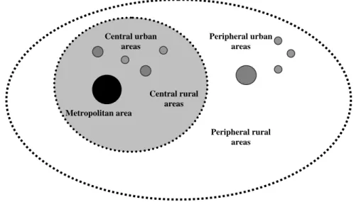
“peripheral” areas. Central and peripheral areas could also be classified taking in account their size. We can begin by distinguishing between urban and rural areas, and urban areas could in turn be classified into different levels according to their size. As a result we obtain five types of regions: Metropolitan Areas, Urban Areas –Central or Peripheral- and Rural Areas –Central or Peripheral.
Figure 1 presents a schematic representation for an idealized national space economy.
The reader will undoubtedly note the resemblance with the classic idealized economic landscapes of Christaller, Lösch, and Von Thünen, all of which posit one metropolis or marketplace at the centre. Thus, Figure 1 posits one metropolis at the centre, but also other smaller “central” urban areas of different population sizes (urban areas close to the metropolis) as well as “central” rural areas (close to the metropolis). Other analogous territories are posited for “peripheral” urban areas, located at some distance
6 from the metropolis, surrounded by corresponding rural places. It is implicitly assumed that urban areas are distributed in accordance with the rank-size rule.
Figure 1: Schematic Representation of the Classification of Spatial Units.
First, we single out the major Spanish cities in order to analyse these separately from the rest. All metropolitan areas (which can include several municipalities) with more than 0.5 million inhabitants are considered as large metropolises (Metropolitan Areas, MA). This limit was established as a result of our observation of Spanish data in the search for the clear divergence in size that exists among Spanish cities. Thus, eleven cases are considered as large metropolises: Madrid, Barcelona, Alicante urban area, Asturias Central Area, Bilbao, Cadiz Bay, Malaga, Murcia and Cartagena Conurbation, Seville, Valencia and Zaragoza. It may make sense to differentiate between Metropolitan Areas with more than 2.5 million inhabitants, that is, Madrid and Barcelona (MA1), and the other metropolitan areas with between 0.5 and 2.5 million inhabitants.
The remaining territories are classified as urban areas (U) when they have between 10,000 and 0.5 million, or as rural areas (R) when they have a population of <10,000 inhabitants. The urban areas are further divided into those >0.1 m (but < 0.5 m) – U1 – and those < 0.1 m (U2).
At the same time, each one of these urban or rural areas may be considered as central (C) or peripheral (P) depending on their distance from a large metropolis. Using the criteria applied by Polése, et al. (2006), all the areas within approximately one hour’s drive of a metropolitan area (with >0.5m inhabitants) are considered as central and the rest as peripheral. This criterion is supported by the evidence accumulated in several
Metropolitan area Central urban
areas
Central rural areas
Peripheral rural areas Peripheral urban
areas
7 studies for different countries. For example, Desmet and Fafchamps (2005) find that the spread of development falls off after about 50 kilometres while Polèse and Shearmur (2004) present similar results for Canada. Thus, the final set of regions is shown in Table 1 and Figure 2 presents a schematic map of the large cities and central, peripheral or ultra-peripheral areas in Spain.
Table 1: Territorial classification by size and position.
Metropolitan areas of more than
2,500,000 million inhabitants (1) MA1
Metropolitan areas of between 500,001
and 2,500,000 inhabitants (2) MA2
Central Urban Areas (no more than one hour drive from a MA)
Peripheral urban areas (more than one hour drive from a
MA)
Urban areas of between 100,001 and
500,000 inhabitants (3) CUA3 PUA3
Urban areas of between 50,001 and
100,000 inhabitants CUA4 PUA4
Rural areas, less than 50,000
inhabitants CRA PARA
Notes:
(1) Madrid and Barcelona.
(2) Alicante, Bilbao, Cadiz Bay, the Central Urban Area of Asturias, Málaga, Murcia and Cartagena Conurbation, Seville, Valencia and Zaragoza.
(3) There are more than 200 municipalities that can be classified as Urban and Central, being the most important ones Alicante, Castellón, Girona, Huelva, Málaga, San Sebastián, Santander-Torrelavega, Tarragona, Vitoria and some of their surrounding municipalities.
8 Figure 2: Map of the Main Spanish Metropolitan Areas and their Respective
Central Areas of Influence.
Main cities (CU/PU) Central area (CU/CR) Insular areas Metropolitan area (MA) Peripheral area (PU/PR)
The employability analysis proposed in this paper will be applied to each of the eight Regions into which we have divided the Spanish territory, where no mention whatsoever is made of the politico-administrative regional frontiers commonly used.
The interpretation of the regression differences will provide us information on the relevance of agglomeration economies and localization effects for employment patterns.
The agglomeration economies are usually divided into two sorts, although this classification in constantly being refined (see Phelps and Ozawa, 2003). First, there are economies linked to the co-location of many firms within the same industry. These economies may be related to a shared labour-force, knowledge spillovers, rapid diffusion of innovations, and stimulation due to the competition between firms (see Rosenthal and Strange, 2001; Porter, 1990; Beardsell and Henderson, 1999).
Secondly, there are economies linked to the co-location of many diverse activities.
Infrastructures such as international airports and highways depend upon a large local market, as do schools, universities and cultural activities. In addition, the presence of a diversity of economic sectors may stimulate the cross-over of ideas, leading to innovations or even to new economic activities (see Jacobs, 1984; Quigley, 1998).
Madrid metropolitan
area Barcelona
metropolitan region Central urban area
of Asturias
Valencia metropolitan area Metropolitan area of
Sevilla
Málaga Cádiz
Bay
Bilbao metropolitan area
Alicante urban area
Murcia and Cartagena urban area Zaragoza
9 This does not mean that larger cities alone will benefit from agglomeration economies:
rather, in keeping with the idea of Phelps el al. (2001) regarding borrowed size and with empirical results from both Canada (Polèse and Shearmur, 2004) and Spain (Polèse, Rubiera and Sheamur, 2007 and Rubiera, 2006), it is the regions within and close to larger cities that will benefit from these advantages. The analysis of the results obtained for the MA1, MA2, CUA1, CUA2 and CRA, as opposed to PUA1, PUA2 or PRA, allow us to measure the real relevance of agglomeration economies in the Spanish case.
3 What Do We Know about Employment Profiles? Main General Conclusions and Types of Databases Used. A Brief Reappraisal
One of the targets of any government is to achieve a high, sustained level of employment. Therefore, the study of the determining factors of employment is an area of great interest for many economists. Regional economics examines the interaction between employment and the economy in general, exploring some of the sub-national characteristics that may result in significant differences in both levels of employment and employment growth rates across space. There are plenty of studies dealing with the analysis of the groups that suffer the highest risk of being unemployed. As their main data sources, these studies typically use the Labour Force Survey elaborated by individual countries, or in the European case, the Living Conditions Survey or the European Household Panel. For all those cases, we are talking about representative statistics at national or regional levels (NUTS III division).
The scarcity of disaggregated information at the local level limits our possibilities for conducting analysis where the size of the geographical units used can be taken into account independently of the administrative region (NUTS III) to which they belong.
Sometimes, this inconvenience is bridged if the data source yields information about the condition of the unit (metropolitan, urban, rural), as is the case of the National Longitudinal Surveys or the Panel Study of Income Dynamics, both in the United States (used among others by Glaeser and Maré, 2001). On other occasions, administrative registered data are used, which includes disaggregated information in geographical terms, but presents some problems related to fact of not having been elaborated for research purposes. (Alonso and del Rio, 2007; Alonso et al., 2008).
Spain is an interesting case study because of its particularities. For a long time the aggregate unemployment rate in Spain was the highest of the European countries, leading to a great number of studies based on the analysis of its explanatory factors
10 (see, for example, Bentolila and Blanchard, 1990; Blanchard and Jimeno, 1995; Dolado and Jimeno, 1997, among others). In addition to the persistence of unemployment, another special characteristic of the Spanish case is the existence of regional disparities that may reflect the existence of regional employment markets, i.e.
differentiated spatial behaviours in response to changes in labour activity (Decressin and Fatás, 1995; Jimeno and Bentolila, 1998). For example, López-Bazo et al. (2005) conclude that in the 1980s such differences were explained mainly by industrial mix and wages, while in the 1990s the differences across provinces in amenities explain the regional dispersion of the employment rates.
Overall, the conclusions of these and other studies highlight the specificity of regional labour markets. The question remains as to whether there may be common factors that contribute to the explanation of the behaviour of these markets, such as, for example, the size of the regional units being considered or their spatial location. One of the main contributions of this study is that, using disaggregated data at local level, we depart from the traditional political-administrative definition of regions (NUTS III) and instead construct a new territorial classification of municipalities which are more economically meaningful (in a sense that we elaborate upon in the next section). Our objective is to use these newly-constructed Regions to analyze differences in the probability of being employed.
4 Database: the Micro-data of the Spanish Census.
One of the main problems in the application of this approach is the major difficulties in obtaining suitable data at local level. The main database for the application of the empirical model is the Spanish Census, administered by the INE (National Statistics Institute of Spain). Although there are partial up-datings every three years, the complete database is only available every ten years. The last two full Spanish censuses available are for 1991 and 2001. We shall use the data from 2001.
The database is based on 5% of the total population that was living in Spain in 2001 according to the Census. As our purpose is to study the influence of the type of municipality in which a person lives (urban vs. rural, central vs. peripheral) on the chances of being employed, from the initial sample those individuals under the age of 16 and over 65 were eliminated. Thus, we are left with a database that includes 1,374,612 working-age individuals, 7.1% of which are foreigners. For each individual we have the following information: age, gender, highest level of studies achieved, marital status (single/married/separate-divorcee/widow), labour situation
11 (employed/unemployed/inactive), number of children above/below the age of 4, and place of birth (domestic/foreign). In our sample, 53.9% of the individuals were working, while 8.9% were searching for a job. The remaining percentage (36.9%) are individuals not economically active.
As regards the spatial units, Spain is divided into seventeen Autonomous Communities, some of which are composed of provinces. There is a national total of 52 provinces, each of which is in turn divided into municipalities in numbers ranging from 35 to 370.
Thus, in 2001 Spain had 8,086 municipalities. A small number of these became municipalities between 1991 and 2001.
As the Census includes information about the municipality where each individual lives, it was possible to identify each territory with our particular classification of Regions (MA1, MA2, CUA1...). The distances to a metropolitan area are calculated using the digital maps of the CNIG (Spanish National Centre for Geographical Research), which offer all the X and Y co-ordinates of the Spanish municipalities. According to our sample, 38.5% of the population had their residence in a metropolitan area (MA1 and MA2), 24.6% live in central areas (CUA1, CUA2 and CRA) and the rest live in the periphery (36.9%) (see table 2).
12 Table 2: Descriptive statistics of the variables.
MA1 MA2 CUA1 CUA2 CRA PUA1 PUA2 PRA. TOTAL Mean S.E. Mean S.E. Mean S.E. Mean S.E. Mean S.E. Mean S.E. Mean S.E. Mean S.E. Mean S.E.
EDUCATIONAL LEVEL
No Studies 0.070 0.255 0.072 0.259 0.061 0.240 0.089 0.285 0.083 0.276 0.065 0.246 0.100 0.300 0.113 0.317 0.082 0.275 Basic Studies 0.432 0.495 0.480 0.500 0.494 0.500 0.538 0.499 0.565 0.496 0.469 0.499 0.550 0.497 0.603 0.489 0.508 0.500 High School 0.166 0.372 0.144 0.352 0.136 0.343 0.126 0.332 0.114 0.318 0.159 0.365 0.128 0.334 0.103 0.303 0.138 0.345 Occupational Studies 0.119 0.324 0.124 0.330 0.139 0.346 0.115 0.319 0.120 0.325 0.113 0.317 0.094 0.292 0.087 0.282 0.112 0.316 University Studies 0.213 0.410 0.179 0.383 0.170 0.375 0.132 0.339 0.118 0.323 0.194 0.396 0.128 0.334 0.094 0.292 0.159 0.366 GENDER
sexo1 0.492 0.500 0.494 0.500 0.494 0.500 0.505 0.500 0.519 0.500 0.491 0.500 0.504 0.500 0.523 0.499 0.502 0.500 sexo2 0.508 0.500 0.506 0.500 0.506 0.500 0.495 0.500 0.481 0.500 0.509 0.500 0.496 0.500 0.477 0.499 0.498 0.500 AGE
<24 0.180 0.384 0.194 0.395 0.189 0.392 0.198 0.398 0.180 0.384 0.196 0.397 0.201 0.401 0.183 0.387 0.190 0.392 25-29 0.135 0.342 0.128 0.334 0.130 0.336 0.128 0.334 0.123 0.328 0.128 0.334 0.125 0.331 0.117 0.322 0.127 0.333 30-44 0.347 0.476 0.348 0.476 0.347 0.476 0.357 0.479 0.364 0.481 0.347 0.476 0.362 0.481 0.354 0.478 0.352 0.478
>45 0.338 0.473 0.330 0.470 0.334 0.472 0.317 0.465 0.333 0.471 0.329 0.470 0.312 0.463 0.346 0.476 0.331 0.471 PLACE OF BIRTH
Local 0.902 0.297 0.942 0.233 0.932 0.252 0.926 0.262 0.940 0.237 0.935 0.246 0.928 0.258 0.946 0.226 0.929 0.256 Foreigner 0.098 0.297 0.058 0.233 0.068 0.252 0.074 0.262 0.060 0.237 0.065 0.246 0.072 0.258 0.054 0.226 0.071 0.256 MARITAL STATUS
Single 0.407 0.491 0.399 0.490 0.401 0.490 0.369 0.483 0.367 0.482 0.416 0.493 0.382 0.486 0.385 0.487 0.393 0.488 Married 0.525 0.499 0.538 0.499 0.534 0.499 0.574 0.494 0.581 0.493 0.518 0.500 0.564 0.496 0.573 0.495 0.548 0.498 Separated/Divorcee 0.048 0.213 0.042 0.200 0.045 0.206 0.038 0.190 0.033 0.179 0.046 0.209 0.033 0.180 0.022 0.148 0.039 0.193 Widow 0.019 0.138 0.021 0.145 0.021 0.142 0.019 0.137 0.019 0.136 0.021 0.142 0.020 0.141 0.020 0.139 0.020 0.140 CHILDREN
With children 0.156 0.363 0.126 0.332 0.135 0.342 0.143 0.350 0.152 0.359 0.115 0.319 0.123 0.329 0.129 0.336 0.136 0.343 No children 0.844 0.363 0.874 0.332 0.865 0.342 0.857 0.350 0.848 0.359 0.885 0.319 0.877 0.329 0.871 0.336 0.864 0.343 With children under 4 0.877 0.328 0.877 0.328 0.874 0.332 0.858 0.350 0.861 0.346 0.881 0.324 0.863 0.344 0.878 0.327 0.872 0.334 No children under 4 0.123 0.328 0.123 0.328 0.126 0.332 0.142 0.350 0.139 0.346 0.119 0.324 0.137 0.344 0.122 0.327 0.128 0.334 With children >4 0.231 0.422 0.194 0.395 0.208 0.406 0.221 0.415 0.230 0.421 0.182 0.386 0.195 0.396 0.191 0.393 0.207 0.405 No children > 4 0.769 0.422 0.806 0.395 0.792 0.406 0.779 0.415 0.770 0.421 0.818 0.386 0.805 0.396 0.809 0.393 0.793 0.405
N 187.282 141.157 38.396 100.942 77.034 98.104 101.803 119.068 863.786
13 5 Modelling Spanish Municipalities Employability Profiles and Basic
Hypothesis.
Our objective is to study the probability of being employed as a function of the specific profile of each individual, and in particular of the type of region or spatial unit in which the person resides. To do so, we use a LOGIT model in which the dependent variable is the probability of being employed, p, which takes value 1 if the individual is employed and value 0 if the individual is unemployed.
The model is as follows:
) '
1 (
1
t
t t
t X
y e
(1)
And their lineal transformation:
t t
t t
t X t
y y y
it
'
ln1 ) (
log (2)
The independent variables, Xi, are those commonly used in studies of individuals’
probabilities of being employed: age (AGE); highest educational level attained (EDL );
marital status (MS); a variable capturing whether the individual was born outside of Spain (FOR); variables capturing whether the individual has children under or above the age of 4 (CHBA4 and CHAA4 respectively); and variables indicating the type of Region where he/she lives (MA1, MA2, CUA1, CUA2, CRA, PUA1, PUA2, PRA). The following table explains the variables used and their sources (see table 3).
14 Table 3: Variables and Data Used in the Empirical Approach.
Variables Database
EMPYN Employed: Yes/No
Dummy variable that provides information about an individual’s labour situation: employed vs non employed.
This variable is constructed using the labour data included in the Spanish Census (2001). The Census is administered by the Spanish National Institute of Statistics, INE.
MA1, MA2
Metropolitan areas: more than 500,000 inhabitants
CUA1, CUA2
Urban (more than 10.000 but less than 500.000 inhabitants) Central areas
PUA1, PUA2
Urban (more than 50.000 but less than 500.000 inhabitants). Peripheral areas
CRA Rural Central areas PRA Rural Peripheral areas
See Table 1. The distances to a metropolitan area are calculated using the digital maps of the CNIG (Spanish National Centre for Geographical Research). Information from the National Government Ministry of Infrastructures and Public Works was used for the delimitation of the metropolitan areas.
AGE Age
For each individual included in the Spanish Census there is information about the year of birth. We aggregate the variable AGE into 4 groups: less than 25, between 25 and 29, between 30 and 44, and more than 44 years of age.
MS Marital Status
The Census (2001) distinguishes between 5 categories:
single, married, widow, separated and divorced. For our purposes we aggregated the separated and divorced individuals.
EDL Educational level
There are 10 different categories for this variable in the Spanish Census (2001). For our purposes we aggregate them in 5 categories: without studies, basic studies, secondary education, vocational training and university education
FORE Foreigner: Yes/No
Dummy variable that establishes if an individual is a foreigner or was born in Spain. The Census (2001) includes information about the country of birth for each individual.
CHBA4 Children under age of 4:
Yes/No
Dummy variable reflecting the existence of children under the age of 4.
CHAA4 Children above age of 4:
Yes /No
Dummy variable reflecting the existence of children above the age of 4.
Spatial unit of the analysis: Spanish municipalities
Given the different behaviour of men and women in the labour market, we have estimated separate models for each which, as we will see, produce interesting differences in the results and their implications.
Specifically, our interest is to test the following hypotheses:
H1: the probability of being employed increases with size
This hypothesis suggests that the concentration of economic activity and the agglomeration economies generated in the largest metropolitan areas increase
15 the opportunities for matching and therefore the chances to be employed, whatever the level of studies or any other characteristic achieved by the worker.
However, this increase should be clearer in those activities which are highly sensitive to the agglomeration economies which coincide with the more qualified or creative jobs.
H2A: the probability of being employed increases with distance for the individuals with a university degree.
H2B: the probability of being employed diminishes with distance for the individuals with occupational formation.
The economic structure and growth are clearly affected by the proximity of a large metropolis. The price of land and the higher salaries that are usually paid in the biggest cities expel some spatial intensive activities less sensitive to agglomeration economies, principally industrial activities, but these activities search for locations that are still close to the metropolis (main market). For this reason, cities and rural areas located close to big cities are expected to produce the highest chances of being employed for individuals with an occupational formation.
On the other hand, when a large metropolis is close to a medium-sized or small city, these are not able to develop business service activities because there is a large and very competitive supply in the nearby metropolis. This implies that the probability of finding a job for individuals with a university degree decreases in the areas close to a large metropolis and, in the same way, increases in all those which are far away from the large metropolis because of the protection by distance.
6 Main Results Discussion.
In this section, we present the main results of the estimated econometric model for the country as a whole and for the regional classification proposed. Separate estimations are made for men and women, as is common in the literature. The basic econometric results are presented in Table 2.
To extract useful conclusions from these results, we calculate the probabilities of being employed for the 24 different plausible profiles. For each profile considered, we also have to distinguish between genders, and each one could live in one of the eight regions defined. Given the large number of results, we will just focus on those we consider more relevant or interesting.
16 Table 2: Employability Model by Region for Men and Women.
a) Men
MA1 MA2 CUA1 CUA2 CRA PUA1 PUA2 PRA Coef. S.E. Coef. S.E. Coef. S.E. Coef. S.E. Coef. S.E. Coef. S.E. Coef. S.E. Coef. S.E.
Married 1,242 *** 0,036 1,237 *** 0,035 1,209 *** 0,076 1,101 *** 0,048 0,736 *** 0,055 1,234 *** 0,043 1,053 *** 0,042 0,716 *** 0,037 separated/divorce 0,526 *** 0,084 0,448 *** 0,091 0,627 *** 0,208 0,197 0,121 0,272 * 0,158 0,452 *** 0,107 0,324 *** 0,124 0,112 0,138 Widow 0,776 *** 0,173 0,863 *** 0,174 0,979 ** 0,380 0,686 *** 0,237 0,465 * 0,263 0,804 *** 0,215 0,876 *** 0,241 0,553 *** 0,198 ref: single
less than 25 -0,463 *** 0,039 -0,306 *** 0,036 -0,275 *** 0,077 -0,385 *** 0,051 -0,483 *** 0,063 -0,344 *** 0,047 -0,286 *** 0,047 -0,390 *** 0,045 30-44 -0,096 ** 0,039 -0,020 0,036 0,130 * 0,078 -0,055 0,052 0,073 0,064 -0,064 0,046 0,013 0,047 0,151 *** 0,043 more than 45 -0,339 *** 0,047 -0,041 0,046 0,004 0,099 -0,169 *** 0,063 -0,060 0,074 -0,026 0,058 -0,048 0,057 -0,007 0,050 ref: 25-30
no studies -0,717 *** 0,055 -1,019 *** 0,054 -0,907 *** 0,117 -1,050 *** 0,071 -1,285 *** 0,085 -0,990 *** 0,065 -1,104 *** 0,063 -1,193 *** 0,065 basic studies -0,243 *** 0,037 -0,352 *** 0,038 -0,197 ** 0,081 -0,320 *** 0,056 -0,251 *** 0,070 -0,278 *** 0,045 -0,270 *** 0,051 -0,429 *** 0,055 occupational studies 0,201 *** 0,048 0,200 *** 0,048 0,375 *** 0,101 0,300 *** 0,074 0,415 *** 0,090 0,360 *** 0,060 0,270 *** 0,070 0,083 0,071 university studies 0,226 *** 0,045 0,320 *** 0,049 0,538 *** 0,109 0,160 ** 0,076 0,275 *** 0,098 0,468 *** 0,059 0,264 *** 0,071 -0,012 0,077 ref: high school
Foreigner -0,563 *** 0,040 -0,417 *** 0,051 -0,327 *** 0,103 -0,446 *** 0,062 -0,440 *** 0,082 -0,340 *** 0,060 -0,495 *** 0,055 -0,491 *** 0,058 children < 4 0,058 0,045 0,008 0,042 -0,086 0,091 -0,063 0,054 0,050 0,065 0,132 ** 0,055 -0,030 0,049 -0,005 0,047 children >5 5 -0,066 ** 0,033 -0,158 *** 0,035 -0,170 ** 0,074 -0,046 0,045 0,037 0,052 -0,037 0,044 0,003 0,042 0,114 *** 0,039 Constant 2,076 *** 0,051 1,644 *** 0,053 1,760 *** 0,110 2,138 *** 0,074 2,245 *** 0,091 1,568 *** 0,065 1,819 *** 0,068 2,056 *** 0,070
b) Women
MA1 MA2 CUA1 CUA2 CRA PUA1 PUA2 PRA
coef S.E. coef S.E. coef S.E. coef S.E. coef S.E. coef S.E. coef S.E. coef S.E.
Married 0,068 ** 0,031 0,271 *** 0,032 0,363 *** 0,067 0,400 *** 0,042 0,090 * 0,051 0,290 *** 0,038 0,368 *** 0,040 0,178 *** 0,038 separated/divorce 0,167 *** 0,051 0,178 *** 0,052 0,241 ** 0,109 0,138 ** 0,070 0,073 0,094 0,217 *** 0,061 0,153 ** 0,070 -0,023 0,082 widow 0,607 *** 0,104 0,588 *** 0,103 0,922 *** 0,257 0,912 *** 0,157 0,433 *** 0,163 0,581 *** 0,124 0,767 *** 0,139 0,674 *** 0,140 ref: single
less than 25 -0,316 *** 0,040 -0,346 *** 0,037 -0,349 *** 0,078 -0,231 *** 0,047 -0,309 *** 0,060 -0,311 *** 0,046 -0,236 *** 0,046 -0,379 *** 0,044 30-44 0,053 0,035 0,206 *** 0,034 0,153 ** 0,072 0,142 *** 0,044 0,222 *** 0,053 0,221 *** 0,042 0,219 *** 0,042 0,267 *** 0,040 more than 45 0,210 *** 0,041 0,532 *** 0,043 0,446 *** 0,090 0,424 *** 0,056 0,520 *** 0,065 0,556 *** 0,052 0,571 *** 0,054 0,672 *** 0,050 ref: 25-30
no studies -0,597 *** 0,056 -0,705 *** 0,061 -0,711 *** 0,136 -0,866 *** 0,075 -1,678 *** 0,083 -0,707 *** 0,073 -0,817 *** 0,068 -1,137 *** 0,065 basic studies -0,463 *** 0,033 -0,488 *** 0,036 -0,460 *** 0,079 -0,526 *** 0,049 -0,606 *** 0,061 -0,421 *** 0,043 -0,301 *** 0,046 -0,453 *** 0,048 occupational studies -0,104 ** 0,041 -0,123 *** 0,042 -0,073 0,091 -0,146 ** 0,058 -0,093 0,073 -0,115 ** 0,051 -0,108 * 0,057 -0,044 0,059 university studies 0,405 *** 0,038 0,396 *** 0,042 0,430 *** 0,093 0,339 *** 0,060 0,265 *** 0,076 0,321 *** 0,049 0,401 *** 0,057 0,197 *** 0,058 ref: high school
foreigner -0,098 ** 0,038 -0,212 *** 0,049 -0,169 * 0,096 -0,113 * 0,060 -0,143 * 0,080 -0,211 *** 0,055 -0,147 ** 0,056 -0,096 0,061 children < 4 -0,476 *** 0,032 -0,438 *** 0,034 -0,474 *** 0,070 -0,569 *** 0,041 -0,477 *** 0,048 -0,415 *** 0,041 -0,404 *** 0,040 -0,495 *** 0,040 children >5 5 -0,178 *** 0,028 -0,152 *** 0,030 0,027 0,061 -0,062 * 0,037 -0,067 0,043 -0,119 *** 0,038 0,019 0,037 -0,020 0,036 constant 1,979 *** 0,044 1,281 *** 0,048 1,491 *** 0,101 1,570 *** 0,063 1,842 *** 0,078 1,322 *** 0,058 1,206 *** 0,061 1,355 *** 0,061
*: significance at 10%; **: significance al 5%; ***: significance at 1%.
17 Given the variety of profiles, lots of different comparisons could be made such as the consequences for employability for a foreigner versus national, or for males versus females. We could also analyse whether marital status has any effect on the chances of being employed or whether occupational studies are a better way to get into the labour market than studying at University. However, as the purpose of this paper is to explore the location patterns of employment given our new definition of a Region (i.e., size and location matters), we will just focus on a few profiles where we observe the most interesting results about the region of residence of an individual. This does not imply that the rest of variables are not important or have no explanatory power.
Results will vary between regions depending on the factors that explain the probability of being employed, i.e. different conclusions for different profiles depending on where individuals live.
As we mentioned above, our hypotheses are that given the existence of agglomeration economies, the probabilities of being employed are expected to decrease for occupational workers and increase with distance for university workers and to grow with size for all type of workers.
In Figure 3, we have represented a married individual (non-foreigner) with no children, aged between 30 and 44 and with university studies. As expected, there is a significant gap in the chances of being employed between central and peripheral areas, confirming that the concentration of economic activity, and therefore employment in jobs requiring higher qualifications, would be in the centres. However, while the relationship between employment and size exists it does not seem to be very strong for this particular profile (individual with University Studies). In the largest metropolitan areas (MA1), a man (woman) with university studies has an almost 97% (92%) chance of being employed, while in a peripheral urban area the probability falls only slightly to 96.1% (89.6%). If the region of residence is peripheral and also rural the figure drops only slightly to 94.8% (88%). The only exceptions to this pattern are the metropolitan areas with >0.5m inhabitants (MA2), where there seems to be a high concentration of unemployment.
On the other hand, the huge gap between the chances of being employed in metropolitan areas 2 (MA2, those with populations between 0.5 and 2.5 m) depending on the level of studies is remarkable. These areas are very peculiar; they have long suffered from unemployment as they are typically areas specialised in traditional industries that have suffered several reconversions in recent decades.
18 Figure 3: Probability of being employed by gender and region.
Profile #1 (married individual, age 30-44, no foreigner, no kids).
Probability of being employed: Gender and Region
85,0%
87,0%
89,0%
91,0%
93,0%
95,0%
97,0%
99,0%
MA1 MA2 CUA1 CUA2 CRA
PUA1 PUA2 PRA
MALE. Central Regions MALE. Peripheral Regions FEMALE. Central Regions FEMALE. Peripheral Regions
However, as high added value activities –and therefore highly qualified jobs– are expected to be concentrated in the central areas, this first overview based on an individual with university studies could be biased.
Obviously, the level of studies has a tremendous different impact in comparisons between central areas and peripheral ones. This can be seen in Figure 4 where we represent the probability of being employed for a profile referred to as #1 (married individual, age 30-44, non-foreigner, no children), having different levels of education and living in different regions. As expected, the higher the level of studies, the higher the probability of being employed in any sort of region. This result holds both for women and for men.
It is relevant to point out that the probability of being employed for somebody holding a university degree versus an individual with occupational studies is slightly higher in metropolitan areas and urban areas of a certain size, either central or peripheral (CUA1 and PUA1). However, the contrary is true for the least populated regions (regions below 100.000 inhabitants, i.e. Urban Areas 2 and Rural Areas), regardless of whether they are considered central or peripheral. In other words, when searching for a job at national level, chances to be employed for somebody with occupational training are higher than the equivalent for an individual with university degree in small central or peripheral regions.
19 Figure 4: Probability of being employed by region, gender and level of studies.
Profile #1 (married individual, age 30-44, no foreigner, no kids)
Employability. Profile #1. NO STUDIES
81,8%
77,6%
61,7%
66,0%
85,4%
89,4%
89,9%
86,3%
92,4%
84,9%
85,2% 85,6%
74,1%
78,5%
72,6%
75,5%
60,0%
65,0%
70,0%
75,0%
80,0%
85,0%
90,0%
95,0%
100,0%
MA1 MA2 CUA1 CUA2 CRA
PUA1 PUA2 PRA
Employability. Profile #1. BASIC STUDIES
94,3%
94,6%
94,8%
92,5%
95,2%
92,4%
93,2%
92,1%
82,4% 83,0% 82,5%
83,7%
78,1% 80,4% 81,6%
79,4%
60,0%
65,0%
70,0%
75,0%
80,0%
85,0%
90,0%
95,0%
100,0%
MA1 MA2 CUA1 CUA2 CRA
PUA1 PUA2 PRA
Employability. Profile #1. HIGH SCHOOL STUDIES
95,5%
96,0%
95,7%
94,6%
96,2%
93,9% 94,7% 94,9%
89,2%
85,3%
88,1% 89,6%
89,1%
85,8%
85,7%
86,2%
60,0%
65,0%
70,0%
75,0%
80,0%
85,0%
90,0%
95,0%
100,0%
MA1 MA2 CUA1 CUA2 CRA
PUA1 PUA2 PRA
Employability. Profile #1. OCCUPATIONAL STUDIES
88,7%
97,0%
97,0%
97,0%
96,8%
95,5%
95,7% 95,9% 95,3%
87,4% 87,7%
83,7%
88,0%
85,3%
84,3%
84,8%
60,0%
65,0%
70,0%
75,0%
80,0%
85,0%
90,0%
95,0%
100,0%
MA1 MA2 CUA1 CUA2 CRA
PUA1 PUA2 PRA
Employability. Profile #1. UNIVERSITY STUDIES
92,1%
96,5%
96,6%
97,4%
96,0%
96,9%
94,8%
95,9%
96,1%
91,8%
92,5%
89,6% 92,0%
88,0%
90,0%
89,6%
60,0%
65,0%
70,0%
75,0%
80,0%
85,0%
90,0%
95,0%
100,0%
MA1 MA2 CUA1 CUA2 CRA
PUA1 PUA2 PRA
On the other hand, the expected negative relationship between employment and the size of the region where the individual lives seems to be strong only for those with no studies or basic studies. In other words, the size of the region does not seem to have a great impact on employability unless non-qualified jobs are sought; in this case, a person has more chances to find a job in larger rather than smaller regions. This might suggest a higher concentration of non-qualified workers in small and medium-sized regions, which increases the competition for the few non-qualified jobs available. In Table 5 we present the concentration index of the level of education for each region.
As we can see, the previous suggestion is confirmed by the data.
Male. Central Regions Male. Peripheral Regions Female. Central Regions Female. Peripheral Regions
20 Table 3: Index of Spatial Concentration of Educational Levels by Region.
Central Regions Peripheral Regions MA1 MA2 CUA1 CUA2 CRA PUA1 PUA2 PRA No Studies 0.85 0.88 0.75 1.08 1.01 0.79 1.22 1.38 Basic Studies 0.85 0.94 0.97 1.06 1.11 0.92 1.08 1.19 High School 1.20 1.05 0.99 0.91 0.83 1.15 0.93 0.74 Occupational Studies 1.06 1.11 1.23 1.02 1.07 1.01 0.84 0.78 University Studies 1.34 1.12 1.06 0.83 0.74 1.22 0.80 0.59
By region, we can observe that differences between the probability of being employed are much less pronounced in metropolitan areas 1 (MA1) than in the remaining regions.
The differences range from 92.4% (male with no studies) to 96.9% (male with university studies), while in the central urban regions with populations between 50,000 and 100,000 (CUA2) these same percentages vary from 89.4% (Male with no studies) to 97% (male with university studies).
As expected, regardless of the level of studies, the chances of being employed are much higher the closer the region where the individual lives is to a metropolitan area.
This holds true for all levels of studies. However, as the employability rate between central (peripheral) urban areas 1 and 2 does not vary significantly, we can suggest that the size of the region is not as relevant as its central-peripheral location. For rural areas, both size and distance seem to be relevant when evaluating employability, i.e., regardless of the level of studies, there are fewer chances to be employed in rural areas as opposed to urban ones and in peripheral areas as opposed to central ones.
Finally, we would like to remark on the contribution of this paper with respect to the differences between employment rates across territories. Researchers have emphasized the role of (administrative) regions, but it is difficult to explain why rates are different (industrial distribution of economic activity, culture, etc.) and which policies can be effective.
Our results point out the relevance of size and distance. The differences across our (economic) regions can be explained by the existence of agglomeration economies. In this sense, similar people living in the same administrative region could have different employment probabilities depending on the municipality in which they live (rural or urban, central or peripheral).
Our results suggest that any government trying to implement a successful employment policy at national or even local level should design several policies addressed to different social groups as well as different areas, abandoning once and for all the
21 administrative definition of a region commonly used. In other words, as well as it is accepted that employment policies for women have necessarily to differ from those designed for men, or that measures to promote hiring young people and their first employment are not the same as those for adults over 45, a new regional approach that takes the size and location of the region into account should be introduced into the agenda.
7 Conclusions.
Most economic studies are conducted at either national or regional levels and it is generally accepted that the conclusions found are applicable at a local level. However, this is not necessarily true. In this paper, we have carried out an analysis at a very local spatial level where the structural, socio-political and geographical characteristics can and in fact do affect the economic results.
Our main objective has been to check whether successful employment profiles are independent of the type of region. We are specifically interested in investigating how the size and location of the region where an individual lives could affect his/her chances of being employed. To do so, we proposed a regional classification based on size, in terms of population, and position, in terms of distance to a large metropolis.
Using this novel classification we use standard econometric tools to study employment profiles (probability of being employed).
Combining the regional variables and the personal characteristics of the individuals (employed or non-employed), a vast amount of possibilities can be analysed. We have observed some interesting differences among the different types of regions constructed.
There is a significant gap between central and peripheral areas in the chances of being employed, confirming the concentration of economic activity, and therefore employment, in the so called “centre.” On the other hand, a relationship between employment and the size of the Region exists but does not seem to be very strong (unless searching for non-skilled jobs). These results hold for all sorts of profiles and for both males and females (although to different degrees).
It should be highlighted that, when searching for a job at national level, the chances of being employed for somebody with occupational training are higher than those for an individual with a university degree only in small central or peripheral Regions. For any other level of qualification, the expected result is confirmed, i.e. the higher your level of studies, the greater the chances of being employed regardless of the Region where you live.
22 A general policy, not adapted to the different sizes and position of the areas, may be not successfully or may even be harmful due to the fact that we should take into account the particular geographical characteristics of each territory. Our results suggest developing policies of occupational formation in medium or small size cities, especially those which are close to large metropolis. In those large metropolises, policies to catch highly qualified workers will be successful. However, this is also a good policy for medium-sized peripheral cities. A general conclusion of our study is that labour policies must be apply at the local level and adapted to the local area characteristics.
23 References.
Alonso, O. and Del Río, C. (2007): “The geographical concentration of unemployment:
A male-female comparison in Spain”, Regional Studies, 42 (3), pp. 401-412.
Alonso, O., Del Río, C. and Toharia, L. (2008): “Un análisis espacial del desempleo por municipios”, Revista de Economía Aplicada, (forthcoming).
Bande, R., Fernández, M. and Montuenga, V. (2008): “Regional unemployment in Spain: Disparities, business cycle and wage setting”, Labour Economics, vol. 15 (5), pp. 885-914.
Blachard and Jimeno (1995): “Structural Unemployment: Spain versus Portugal”, American Economic Review, 85 (2), pp. 277-292.
Behrens, K. y Thisse, J. F. (2007): “Regional Economics: A New Economic Gaography Perspective”, Regional Science and Urban Economics, 37, pp. 457-465.
Bearsell, M. and Henderson, V. (1999): “Spatial evolution of the computer industry in the USA”, European Economic Review, 43, 431-56.
Bentolila, S. and Blanchard, O.J. (1990): “Spanish unemployment”, Economic Policy, 10, pp. 233-281.
Castells, M. (1976): La Cuestión Urbana, Siglo XXI Editores, México D.F.
CNIG (2001): Mapas digitales de los municipios españoles, Centro Nacional de Información Geográfica, Ministerio de Fomento.
Coffey, W. J. and Polèse, M. (1988): “La Transformation de L´espace Économique Canadien: ¿Assistons-nous à un Mouvement Centre-Péripherie?”, Revue d'économie régionale et urbaine, 1.
Decressin, J. and Fatás, A. (1995): “Regional labor market dynamics in Europe”, European Economic Review, 39, pp. 1627-1655.
Desmet, K. and Fafchamps, M. (2005): “Changes in the spatial concentration of employment across US countries: a sectoral analysis (1972-2000)”, Journal of Economic Geography, 5, 261-284.
Dolado, J.J. and Jimeno, J.F. (1997): “The causes of Spanish unemployment: A structural VAR approach”, European Economic Review, 41 (7), pp. 1281-1307 Duraton, G. and Puga, D. (2002): “Diversity Specialization in Cities: Why, Where and
Does it Matter”, McCann, P. (Ed.): Industrial Localization Economics, pp. 151-186, Cheltenham.
Fujita M., Krugman P. and Venables A. (1999): The Spatial Economy: Cities, Regions and International Trade, Cambridge, MA, MIT Press.
Glaeser, E. L., Scheinkman, J. and Shleifer, A. (1995): “Economic Growth in a Cross- Section of Cities”, Journal of Monetary Economics, 36, pp.117-143.
Glaeser, E.L. (1998): “Are Cities Dying?”, Journal of Economics Perspectives, 12, 2, pp.
139-160.
Glaeser E. and Maré D. (2001): “Cities and skills”, Journal of Labor Economics, 19, pp.
316–342.
Hall, P. (1999): Cities and civilization, Phoenix Giant, London.
Henderson, J.V. and Thisse, J.F. (1997): “On the Strategic Community Development," CEPR Discussion Papers 1550, C.E.P.R. Discussion Papers.
24 INE (2001): Censo de Población, 2001, Instituto Nacional de Estadística
(http://www.ine.es).
INE (1991): Censo de Población, 1991, Instituto Nacional de Estadística (http://www.ine.es).
Jacobs, J. (1984): Cities and the wealth of nations, Vintage, New York.
Jimeno, J.F. and Bentolila, S. (1998): “Regional unemployment persistence: Spain 1976–94”, Labour Economics, 5, pp. 25–51.
López-Bazo, E., del Barrio, T. and Artís, M. (2005): “Geographical distribution of unemployment in Spain”, Regional Studies, 39 (3), pp. 305-318.
Parr, J. (2002): “Agglomeration economies: ambiguities and confusions”, Environment and Planning A, 34, pp. 717-731.
Phelps, N., Fallon, R. and Willians, C. (2001): “Small firms, borrowed size and the urban-rural shift”, Regional Studies, 53 (7), pp. 613-624.
Phelps, N. A. and Ozawa, T. (2003): “Contrasts in agglomeration: proto-industrial, industrial and post-industrial forms compared”, Progress in Human Geography, 27, pp. 583-604.
Porter, M. (1990): The competitive advantage of nations, Free Press, New York.
Polèse, M. and Champagne, E. (1999): “Location matters: Comparing the distribution of economic activity in the Mexican and Canadian urban systems”, International Journal Science Review, 22, pp. 102-132.
Polèse, M. (2005): “Cities and National Economic Growth: A Reappraisal”, Urban Studies, 42 (8), pp. 1429-1451.
Polèse, M. (2009): The Wealth and the Poverty of Regions: Why Cities Matters, University of Chicago Press, Chicago.
Polèse, M. and Shearmur, R. (2004): “Is Distance Really Dead? Comparing the Industrial Location Patterns over Time in Canada”, International Regional Science Review, 27 (4), pp. 1-27.
Polése M., Shearmur, R. and Rubiera, F. (2007): “Observing regularities in location patters. An analysis of the spatial distribution of economic activity in Spain”, European Urban & Regional Studies, 14 (2), pp. 157-180.
Rosenthal, S.S. and William C. S. (2001): “The determinants of agglomeration”, Journal of Urban Economics, 50 (2), pp. 191–229.
Rubiera, F. (2006): Ciudades, Crecimiento y Especialización Territorial. Dinámicas Espaciales de Concentración del Empleo y la Población en España. Consejo Económico y Social. Madrid (España).