an input-output model of migration and commuting

CITIES TO LIVE OR TO WORK IN: AN INPUT-OUTPUT MODEL OF MIGRATION AND COMMUTING

ANA VIÑUELA

ESTEBAN FERNÁNDEZ-VÁZQUEZ

FUNDACIÓN DE LAS CAJAS DE AHORROS DOCUMENTO DE TRABAJO

Nº 668/2011

De conformidad con la base quinta de la convocatoria del Programa de Estímulo a la Investigación, este trabajo ha sido sometido a eva- luación externa anónima de especialistas cualificados a fin de con- trastar su nivel técnico.

ISSN: 1988-8767

La serie DOCUMENTOS DE TRABAJO incluye avances y resultados de investigaciones dentro de los pro- gramas de la Fundación de las Cajas de Ahorros.

Las opiniones son responsabilidad de los autores.

CITIES TO LIVE OR TO WORK IN: AN INPUT-OUTPUT MODEL OF MIGRATION AND COMMUTING

Ana Viñuela*

Esteban Fernández-Vázquez**

Abstract

Madrid and Barcelona have traditionally been recipient provinces for in- migration in Spain. Since mid 1990s the inflows of workers into the two main Spanish cities have increased dramatically reinforced by the arrival of immigrants. These inflows should have affected the original distribution of population and labor force within the city itself and its surrounding areas, i.e. the metropolitan area. Two opposite forces are at play: the existence of agglomeration economies suggests a concentration of economic activity -and therefore jobs- in the city, while the agglomeration diseconomies associated with the arrival of new workers suggest a runaway of residents to some other places more attractive to live in but still close to the city.

Using the latest Spanish Census available -from 2001- and working at municipal level, this paper explores the effects that the arrival of new workers (either nationals or foreigners) has had

areas. The input-output model suggested includes both migration and commuting flows, which allows us to analyze the displacement effect -and its subsequently distribution of workers- as well as the commuting patterns, i.e.

distribution of residents, within the two main Spanish metropolitan areas.

Keywords: input-output tables and analysis, regional migration, commuting,

regional and urban structure, agglomeration economies.

JEL classification: D57, R23, R12

* Applied Economics Department. Universidad de Oviedo. Facultad de Economía y Empresa.

Campus del Cristo s/n. 33006. Oviedo. SPAIN

** Applied Economics Department. Universidad de Oviedo. Facultad de Economía y Empresa.

Campus del Cristo s/n. 33006. Oviedo. SPAIN. E-mail: [email protected]

2

The intensity of in-migration flows, both from abroad and from other regions, to the provinces of Madrid and Barcelona (the most populated Spanish provinces) has been growing since the beginning of the 1990s. In the period that goes from 1991 to 2001, Spain registered around 3,000,000 migration movements of workers, being the destination of more than 35% the provinces of Madrid and Barcelona (Barcelona received 15.91% and Madrid 20.51%). Our hypothesis is that these inflows have affected somehow the original distribution of population and labor force within the municipalities that respectively comprise these provinces.

When some migration inflows are received, two opposite forces are at play: it enhances city size, which can trigger the agglomeration economies leading to a concentration of economic activity -and therefore jobs- in the city. On the other hand, the arrival of new workers can generate diseconomies associated that pushes previous residents to some other places more attractive to live in.

Using the latest Spanish Census available -from 2001- and working at municipal level, this paper explores the effects that the arrival of new workers (either nationals or foreigners) has had within Madrid and Barcelona metropolitan areas. The input-output model suggested includes both migration and commuting flows, which allows us to analyze the displacement effect -and its subsequently distribution of workers- as well as the commuting patterns, i.e.

distribution of residents, within the two main Spanish metropolitan areas.

3 The paper is organized as follows: Section 2 describes the bases of a multiregional model that studies the effects of immigration from the periphery to the core by means of a multipliers matrix. The proposed methodology is based on the input-output migration model developed in Fernandez-Vazquez

(2010). This model analyzed the effect on internal migration patterns as a consequence of immigration. Section 3 explains how the model can be extended to the study of the distribution of jobs across the set of regions, by incorporating information of commuting flows. In section 4, a typology of cities is suggested by means of an indicator that combines the two models introduced in the previous sections. Section 5 presents an empirical application of the methodology proposed to the provinces of Madrid and Barcelona using microdata from the most recent Census. Finally, Section 6 presents the concluding remarks of the paper.

1.

From the assumption that foreign immigration affects internal mobility by displacing population (national in-migration), the multiregional input-output model proposed on Fernández-Vázquez et al. (2010) quantifies the effects that these arrivals generate on the migration patterns in the core itself. It is important to note that this methodology is not an attempt to investigate the causal relationships between internal migrations and some explanatory variables. Instead, we suggest a type of analysis that shares many common points with the so-called Garin-Lowry models. Originally proposed by Lowry (1964) and Garin (1966), these models have been frequently used to explain the allocation of population and labor among different locations from an initial push of basic employment, see for example, McGill (1977), Batty (1983), Guldman and Wan (1998), Jun (2005).

The point of departure for the analysis will be to consider a set of N

geographical units that experience the spatial re-allocation of some part of their

workforce in a given period of time. For the sake of simplicity, in this chapter we

will specifically consider a set of N cities (C), where some inter-city migration

4 flows are observed. In this situation, the following table reflects the migration flows among these cities

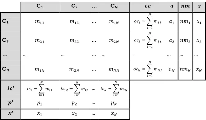
Table 1. Matrix of migrations among N cities.

C1 C2 … CN

C1 𝑚₁₁ 𝑚₁₂ … 𝑚_1𝑁

C2 𝑚₂₁ 𝑚₂₂ … 𝑚_2𝑁

… … … … …

CN 𝑚_1𝑁 𝑚_2𝑁 … 𝑚_𝑁𝑁

where a typical element

denotes the number of workers that migrate from city i to another city j. For any city j considered, the net inflow of migrants (

) received will be:

𝑛𝑚_𝑗 =�𝑖𝑐_𝑗+𝑝_𝑗� − �𝑜𝑐_𝑗+𝑎_𝑗�

(1) Equation (1) defines the net inflow of workers for each type of city. In other words, this variable is defined as the difference between the arrival of new workers - consisting of the in-migration coming from other cities (

) plus the workforce coming from the periphery (

), i.e., either peripheral cities or from another country - and the outflows of people given by the out-migration to other cities located into the core (

) as well as the out-migration to other cities (

).

Note from Table 2 that it is possible to obtain

as the column sum

. Likewise, the out-migrations from city

) can be obtained as the row sum

𝑗=1

. Conversely, the migration flows to and from other cities (

and

, respectively) do not appear in Table 2 but they can be included in it jointly with net migration (

) in order to construct a new table that fulfils the demographic identity (1), and where the row sums equal the column sums. With this purpose in mind, let us define a N×1 vector

, where a typical element

1 The traditional matrix algebraic notation is applied: bold uppercases denote matrices, bold lowercases (column) vectors and italic lowercases scalars. A prime indicates transpose.

5 shows the inflows arriving to municipality j. Note that the elements of this vector can be defined as the sum

, or alternatively as

, from equation (1).

This equivalence holds also when considering the whole vector:

𝒙^′ =𝒊𝒄^′+𝒑′

(2a)

𝒙= 𝒏𝒎+ [𝒐𝒄+𝒂]

(2b)

Consequently, Table 1 can be modified in the following way in order to verify that the row and column sums are both equal to vector x.

Table 2. Migration flows in an inflow-outflow table.

C1 C2 … CN 𝒐𝒄 𝒂 𝒏𝒎 𝒙

C1 𝑚₁₁ 𝑚₁₂ … 𝑚_1𝑁 ^𝑜𝑐1=� 𝑚_1𝑗

𝑁 𝑗=1

𝑎₁ 𝑛𝑚₁ 𝑥₁

C2 𝑚₂₁ 𝑚₂₂ … 𝑚_2𝑁 ^𝑜𝑐2=� 𝑚_2𝑗

𝑁 𝑗=1

𝑎₂ 𝑛𝑚₂ 𝑥₂

… … … … … ^… ... ... ...

CN 𝑚_1𝑁 𝑚_2𝑁 … 𝑚_𝑁𝑁 ^𝑜𝑐𝑁=� 𝑚_𝑁𝑗

𝑁 𝑗=1

𝑎_𝑁 𝑛𝑚_𝑁 𝑥_𝑁 𝒊𝒄’ _{𝑖𝑐1=� 𝑚𝑖1}

𝑁 𝑖=1

𝑖𝑐12=� 𝑚𝑖2 𝑁 𝑖=1

… 𝑖𝑐𝑁=� 𝑚𝑖𝑁 𝑁

𝑖=1

𝒑’ 𝑝₁ 𝑝₂ ... 𝑝_𝑁

𝒙’ 𝑥1 𝑥2 ... 𝑥𝑁

Some assumptions are required in order to explain

model. One basic assumption is that the arrival of new workers from the periphery (vector

Additionally, from Table 3 we will define a coefficient

𝑖

. These

coefficients measure the number of workers that move from city

relative to the total number of workers received in i (including those coming from

6 other cities out of the system). If, for instance,

, this would imply that for each 100 workers received in city

coefficients

are a sort of “rate of displacement” that defines the reaction of city i when it receives new workers. The basic idea behind these

is that the arrival of these new workers to one city produces some “diseconomy” (e.g.:

rises in housing prices, traffic congestion, etc.) that encourages some of the previous residents to migrate.

Another essential assumption of the model is that the

coefficients are assumed to be fixed in the short run. The matrix

contains all the

coefficients for the N cities included in the model:

𝑩=�

𝑏₁₁ 𝑏₁₂

𝑏₂₁ 𝑏₂₂ . 𝑏_1𝑁 . 𝑏_2𝑁

. .

𝑏_𝑁1 𝑏_𝑁2 . . . 𝑏_𝑁𝑁

�

(3)

As a result, the vector of workers coming from other cities (

expressed as:

𝒊𝒄^′=𝒙^′𝑩= [𝑥₁ … 𝑥_𝑁]�

𝑏₁₁ 𝑏₁₂

𝑏₂₁ 𝑏₂₂ . 𝑏_1𝑁 . 𝑏_2𝑁

. .

𝑏𝑁1 𝑏𝑁2

. . . 𝑏𝑁𝑁

�= [𝑖𝑐₁ … 𝑖𝑐_𝑁]

(4)

and equation (2a) can be rewritten in terms of

as:

𝒙^′ =𝒊𝒄^′+𝒑^′=𝒙^′𝑩+𝒑′

(5)

Suppose that the group of N cities receives in a given period a vector of

new workers

of the labor out to another one of the N cities. This will generate a new round of

movements in the system equal to

, which will further displace a part of the

7 workers equal to

process of obtaining the new vector of incoming workers

𝒙’ =𝒑’ +𝒑’𝑩+𝒑’𝑩^𝟐+𝒑’𝑩^𝟑+⋯=𝒑’[𝑰+𝑩+𝑩^𝟐+𝑩^𝟑+⋯]

(6) where I is the identity matrix. Under certain mathematical conditions, (6) can be written as:

𝒙’ = 𝒑’[𝑰 − 𝑩]^−𝟏

(7)

Equation (7) explains how the arrival of new workers to the cities

changes due to variations in the vector of workers coming from peripheral cities

The idea underlying equations (3.6) and (3.7) is that any increase in the movement of workers from the periphery to a city situated in the core, apart from the direct impact that it has on this specific city, generates a set of indirect effects on the entire system of N cities that turns out to be larger than the initial shock.

In the framework defined by the previous model, the elements of the matrix

play a crucial role. The structure of this matrix is:

[𝑰 − 𝑩]^−𝟏= �

𝛽11 𝛽12

𝛽21 𝛽22

. 𝛽1𝑁

. 𝛽2𝑁

. .

𝛽_𝑁1 𝛽_𝑁2 . . . 𝛽_𝑁𝑁

�

(8)

where the element

shows the variation in the number of workers that arrive to the city j due to the arrival of one additional worker to the city i.

This means that

can be interpreted as an approximation to the following derivative:

𝛽_𝑖𝑗 =𝑑𝑥𝑗

𝑑𝑝_𝑖

(9)

2 Readers accustomed to the input-output literature will easily see the analogy of this proposal with the so-called Gosh input-output model (see Dietzenbacher, 1997).

8 It is important to note that even if there are no direct migration flows between cities i and j,

might still be different from zero given that it also measures the indirect effects. For example, the migration from the periphery of workers to city

from h move to the city j.

The previous model (7) explains how workers allocate and reallocate their place of residence across the system of N cities (vector

) given the initial stimulus of new entries of workers. It is important to highlight that it models the choice of residence of the workers, which may not be the same place where they have their jobs. This is a significant difference because while it is possible that a city i displaces workers to another city

produced by additional dwellers which turn city

live in, these workers might keep their jobs in the original city i because it is still attractive to work there. In other words, the model allows the possibility of commuting given that the location of homes and jobs might not be in the same city.

2. The role of commuting

In a fashion similar to the previous section, the commuting flows between the N

cities can be represented in the following table (Table 3), where the cities of

origin are displayed by rows and the destinations are shown by columns.

9

C1 C2 … CN 𝒙

C1 𝑓11 𝑓12 … 𝑓1𝑁 𝑥1

C2 𝑓₂₁ 𝑓₂₂ … 𝑓_2𝑁 𝑥₂

… … … … … ...

CN 𝑓1𝑁 𝑓2𝑁 … 𝑓𝑁𝑁 𝑥𝑁

𝒍 𝑙1 𝑙2 ... 𝑙𝑁

𝑓𝑖𝑗

stands for the flow of workers in a given period of time that arrived to live in the city i but commute to the city

workers that live and work in the same city. Note that

and that

∑^𝑁_𝑖=1𝑓_𝑖𝑗 =𝑙_𝑗

, where

is the total number of jobs occupied by the vector of workers

that are allocated in city j.

For the sake of convenience, we will work with proportions of commuters instead of working directly with flows. These proportions will be defined as

𝑖

and measure the fraction of workers who live in city i but work in city

For example,

means that 25% of the workers who migrated to city i commute to city

matrix of proportions

, it is straightforward to see that:

𝒍′=𝒙′𝑪

(10)

Equation (10) links the entries of workers that live in the system of N

cities (

that this equation is simply a mathematical expression that relates the place of

residence to the location of the jobs. However, by combining equations (7) and

(10) we can construct the following model that explains the spatial allocation of

10 the new jobs from the exogenous shock produced by the arrival of workers from the periphery to the core (

𝒍^′ =𝒙^′𝑪=𝒑^′[𝑰 − 𝑩]^−𝟏𝑪

(11)

Equation (11) models the spatial location across the core of the economic activity (new jobs) generated as a consequence of new workers coming to live in the set of cities. The idea is that workers from the peripheral cities (

) arrive to the cities, which produces a sequence of indirect effects through migrations - matrix

- that subsequently implies a specific distribution of jobs - matrix

. The whole sequence of multiplier effects on the generation of jobs is given by the product of the matrices

and

. Letting

, equation (11) can be written as:

𝒍^′ =𝒑^′𝑴^∗

(12)

where:

𝑴^∗ = �

𝜇11 𝜇12

𝜇21 𝜇22

. 𝜇1𝑁

. 𝜇2𝑁

. .

𝜇_𝑁1 𝜇_𝑁2 . .

. 𝜇_𝑁𝑁�

(13)

and a typical element

shows the variation in the number of jobs in the city j given by the arrival of one additional worker to city i. Note that these elements are given by the sums

, so that in more detail we have:

𝜇_𝑖𝑗 = � 𝛽_𝑖ℎ𝑐_ℎ𝑗

𝑁 ℎ=1

= �𝑑𝑥ℎ

𝑑𝑝_𝑖 𝑓_ℎ𝑗

𝑥_ℎ

𝑁 ℎ=1

=𝑑𝑥1

𝑑𝑝_𝑖 𝑓_1𝑗

𝑥₁ +𝑑𝑥2

𝑑𝑝_𝑖 𝑓_2𝑗

𝑥₂ +⋯+𝑑𝑥𝑁

𝑑𝑝_𝑖 𝑓_𝑁𝑗

𝑥_𝑁 (14)

The idea underlying the

elements is that they comprise a two-stage process:

the entries of workers from the periphery to city i generate a variation - through the whole round of indirect effects captured in

- in the inflows of labour to city

ℎ

of which are going to commute to city

11 considered together and summed across all the cities h,

can be taken as an approximation to the derivative:

𝜇𝑖𝑗 = 𝑑𝑙𝑗

𝑑𝑝𝑖 (15)

We may be interested in studying the capability of each city of getting the jobs that are generated by the entrance of new workers in the cities. In other words, we could be interested in estimating how many jobs will locate to city j when all the cities receive one additional worker coming from the periphery. Note that this number can be obtained by the sum

and it can be written as:

𝜇·𝑗 = ∑𝑁 𝜇𝑖𝑗

𝑖=1 = ∑ _𝑑𝑝^𝑑𝑙𝑗

𝑖 𝑁𝑖=1 = _𝑑𝑝^𝑑𝑙𝑗

1+_𝑑𝑝^𝑑𝑙𝑗

2+⋯+_𝑑𝑝^𝑑𝑙𝑗

𝑁

(16)

Relatively large values of

would indicate that city

more jobs than the average city when workers coming from the periphery migrate to the core.

3. Classifying the cities: places to work or to live in?

The elements of matrices (8) and (13) remark the effect that the arrivals of

workers from out of the system (vector

) have both on the residential (vector

)

and job location (vector

) patterns. It seems logical to expect that along the set

of N cities, some of them experience a relatively larger effect on one of the two

possible effects. For example, the new workers might decide to live in some

specific location i but commute to a different one because there are better

opportunities to work there. This would turn out in a large effect on

but a

small effect on

. Conversely, in one city i we could observe a huge generation

of jobs as a consequence of the exogenous shock of vector

, but the number

of workers who have their residence there might be small –because of high

prices of housing, for example- and consequently we would have big effects on

but smaller on

.

12 From this simple idea, we can define a measure of “net demand of commuters”

for a city

, which compares the number of jobs that are located in that city with the number of workers that live there. If this difference is positive, this means that the city i would require commuters from other areas in order to fill the jobs that are not taken by the local workers. In other words, this would be a signal that would indicate that city i is attractive for working but not for living. The opposite would happen if this difference is negative.

If we compute this difference for the whole set of N cities, we would have:

𝒅′=𝒍′ − 𝒙′,

(16)

and taking into account the equations (11) and (7):

𝒅′=𝒍^′− 𝒙^′= 𝒑^′[𝑰 − 𝑩]^−𝟏𝑪 − 𝒑^′[𝑰 − 𝑩]^−𝟏 =𝒑^′[𝑰 − 𝑩]^−𝟏[𝑪 − 𝑰]

(17) If we denote with

the matrix obtained by the product

the previous equation can be written as:

𝒅′=𝒑^′𝚫

(18)

Where:

𝚫= �

𝛿₁₁ 𝛿₁₂

𝛿₂₁ 𝛿₂₂ . 𝛿_1𝑁 . 𝛿_2𝑁

. .

𝛿𝑁1 𝛿𝑁2

. . . 𝛿𝑁𝑁

�

(19)

And a typical element

shows the variation in the requirement of commuters in the central city j produced by one additional worker migrating to city

Considering that each element

comes from the product given by

, its expression is:

𝛿_𝑖𝑗 =� 𝛽_𝑖ℎ𝑐_ℎ𝑗

𝑁 ℎ≠𝑗

+𝛽_𝑖𝑗�𝑐_𝑗𝑗 −1�

(20)

13 Note that the element

will be positive if:

� 𝛽𝑖ℎ𝑐ℎ𝑗 𝑁

ℎ≠𝑗

>𝛽𝑖𝑗�𝑥𝑗− 𝑓𝑗𝑗

𝑥𝑗 �

i.e., if the arrival of new workers to city i produces an increase in the commuters to

larger than the increase in the number of workers that commute from j (

). Oppositely, the variation in

could cause an increase in the workers that have their residence in other city h and commute to work in j smaller than the growth in the workers living in j but commuting to anywhere else. In such a case,

would be negative, which would indicate that the rise in the immigrant workers form the periphery arriving to city i produce an increase in the residents rather than in the jobs in j. If, on the contrary,

is positive, the additional workers coming from the periphery to city i would enhance the jobs located in j to a greater extent that the workers residing there.

From these

multipliers it would be possible to classify the cities in two different types: those that are capable to attract comparatively more jobs than residents -job attracting- when new workers enter in the system of N cities and those where the opposite happens –resident absorbing-. This information can be obtained by the sum

. In general terms, the following vector contains these sums for all the cities:

𝜹^′= 𝒆′𝚫

(22)

When an element

of the vector

can be classified as “job attracting”. If, on the contrary,

is negative then the

city j would be “resident absorbing”.

14

1991-2001.

This section applies the aforementioned methodology to develop a model of migration and commuting flows between 1991 and 2001 for Madrid and Barcelona using the data from the last National Census. As explained above, in Spain internal mobility has traditionally not been very high, but it has recently experienced a considerable increase together with a remarkable rise in the reception of immigrants.

The data required for the model have been obtained taking a sample of microdata extracted from the most recent Censo de Población y Viviendas - Population and Housing Census (PHC) - compiled by the Spanish National Statistical Institute for 2001. The sample comprises approximately 5% of the whole census, corresponding to a sample size of around two million people.

The information contained in the survey includes the part of population who were working in 2001, the municipality where they were working and the municipality where they were living. Moreover, information about the municipality where they lived in 1991 is also available. From the data observable, we can identify 27 municipalities in Madrid and 39 in Barcelona.

Some of the municipalities (those smaller than 20,000 inhabitants) are not identifiable since they are too small and data for them are not disclosed in the Census for privacy reasons.

Tables 4a and 4b show the cities included in both models ranked according to their population in 2001:

3 We suspect that the impact of the no consideration of these municipalities in our study is limited for the case of Madrid, since they represent less than 9% of population. In the case of Barcelona, however, it could be more problematic because the population living in these municipalities represent around 20% of the population in 2001.

15

City Population City Population

Madrid 2,938,723 Majadahonda 50,683

Móstoles 196,524 Collado Villalba 47,001

Fuenlabrada 182,705 Aranjuez 40,797

Alcalá de Henares 176,434 Tres Cantos 36,927

Leganés 173,584 San Fernando de Henares 36,244

Alcorcón 153,100 Rivas-Vaciamadrid 35,742

Getafe 151,479 Colmenar Viejo 35,181

Torrejón de Ardoz 97,887 Arganda del Rey 33,432

Alcobendas 92,090 Valdemoro 33,169

Parla 79,213 Pinto 31,340

Coslada 77,884 Boadilla del Monte 27,443

Pozuelo de Alarcón 68,214 Galapagar 25,559

Las Rozas de Madrid 63,385 Villaviciosa de Odón 22,564 San Sebastián de los Reyes 61,884

Table 4b. Municipalities for Barcelona province included in the model

City Population City Population

Barcelona 1,503,884 Sant Feliu de Llobregat 40,042

Hospitalet de Llobregat (L´) 239,019 Gavà 39,815

Badalona 205,836 Igualada 33,049

Sabadell 183,788 Vic 32,703

Terrassa 173,775 Sant Adrià de Besòs 31,939

Santa Coloma de Gramenet 112,992 Vilafranca del Penedès 31,248

Mataró 106,358 Ripollet 30,235

Cornellà de Llobregat 79,979 Sant Joan Despí 28,772

Sant Boi de Llobregat 78,738 Montcada i Reixac 28,295

Manresa 63,981 Barberà del Vallès 26,428

Prat de Llobregat (El) 61,818 Premià de Mar 26,334

Rubí 61,159 Sant Vicenç dels Horts 24,694

Sant Cugat del Vallès 60,265 Sant Pere de Ribes 23,134

Viladecans 56,841 Martorell 23,023

Vilanova i la Geltrú 54,230 Sant Andreu de la Barca 21,933

Cerdanyola del Vallès 53,343 Pineda de Mar 21,074

Granollers 53,105 Masnou (El) 20,678

Mollet del Vallès 47,270 Molins de Rei 20,639

Castelldefels 46,428 Santa Perpètua de Mogoda 20,479

Esplugues de Llobregat 45,127

16 We have applied the three previous input-output models to the municipalities of both provinces. Firstly, from the tables of migration flows, we have divided these flows by the respective vector of total inflows

to compute the coefficient matrix

. This allows obtaining the inverse

composed by the

multipliers. They quantify how many workers municipality i displaces directly and indirectly to city j as a consequence of the arrival of new workers from outside of the province to city i. If we calculate the sums

, we will have an indicator that measures the amount of workers displaced from region i to other central regions. Figures 1a and 1b show these indicators for both provinces:

Figure 1a. Population displacement multiplier (𝜷𝒊·) for Madrid province

0,00 2,00 4,00 6,00 8,00 10,00 12,00 14,00 16,00 18,00

Madrid Móstoles Fuenlabrada Alcalá de Henares Leganés Alcorcón Getafe Torrejón de Ardoz Alcobendas Parla Coslada Pozuelo de Alarcón Rozas de Madrid (Las) San Sebastián de los Reyes Majadahonda Collado Villalba Aranjuez Tres Cantos San Fernando de Henares Rivas-Vaciamadrid Colmenar Viejo Arganda del Rey Valdemoro Pinto Boadilla del Monte Galapagar Villaviciosa de Odón

17

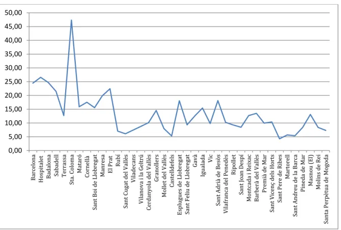
Figure 1b. Population displacement multiplier (𝜷𝒊·) for Barcelona province

The charts above show that there seems to pattern relating city size and the number of workers that each city displaces to other locations. We can see how for middle-size cities like Móstoles,

multipliers than for the city of Madrid itself. Something similar happens for the province of Barcelona, where municipalities like Hospitalet and

present larger estimates than the city of Barcelona. Apart from these cases that can be considered as exceptions, the graphs suggest a general negative relationship between the value of the

multipliers and the size of the municipalities studied.

Besides the data on residence mobility between 1991 and 2001 the microdata in the census also informs about the commuting patterns in 2001, because for each person included in the sample, the municipality of residence and also the location of the job was registered. This allows us to obtain a matrix that contains the commuting trips among the N cities, with the same structure as the previous

0,00 5,00 10,00 15,00 20,00 25,00 30,00 35,00 40,00 45,00 50,00

Barcelona Hospitalet Badalona Sabadell Terrassa Sta. Coloma Mataró Cornellà Sant Boi de Llobregat Manresa El Prat Rubí Sant Cugat del Vallès Viladecans Vilanova i la Geltrú Cerdanyola del Vallès Granollers Mollet del Vallès Castelldefels Esplugues de Llobregat Sant Feliu de Llobregat Gavà Igualada Vic

Sant Adrià de Besòs Vilafranca del Penedès Ripollet Sant Joan Despí Montcada i Reixac Barberà del Vallès Premià de Mar Sant Vicenç dels Horts Sant Pere de Ribes Martorell Sant Andreu de la Barca Pineda de Mar Masnou (El) Molins de Rei Santa Perpètua de Mogoda

18 Table 3. This way, the proportions of commuters defined as

i

will be computed to obtain the matrix

. This matrix will be used to replicate the equation (11) for our study case and compute the multiplier matrix

, where a typical element μ

quantifies the variation in the jobs located in j generated by the arrival of one additional worker to city i. Now, we will focus our analysis in the number of jobs located on city j when all the municipalities in the province receive one additional worker coming from outside. Figures 2a and 2b show the sums μ

μ

. As explained in section 3, large values of

indicate that city j attracts comparatively more jobs than the average.

Figure 2a. Job location multiplier (𝛍·𝐣) for Madrid province

0 20 40 60 80 100 120

Madrid Móstoles Fuenlabrada Alcalá de Henares Leganés Alcorcón Getafe Torrejón de Ardoz Alcobendas Parla Coslada Pozuelo de Alarcón Rozas de Madrid (Las) San Sebastián de los Reyes Majadahonda Collado Villalba Aranjuez Tres Cantos San Fernando de Henares Rivas-Vaciamadrid Colmenar Viejo Arganda del Rey Valdemoro Pinto Boadilla del Monte Galapagar Villaviciosa de Odón

19

Figure 2b. Job location multiplier (𝛍_·𝐣) for Barcelona province

The results in the previous graphs highlight the relevance of the big cities regarding the number of new jobs they are able to attract. In this two provinces characterized by two enormous cities surrounded by other municipalities much smaller in size, the arrivals of new workers displaces more residents than the average from these big municipalities but they manage to keep on them most of the jobs. All in all, a general idea would be that the immigration of labour force pushes workers from living in big cities to reside in the smaller locations situated in the province. However, the large metropolises manage to keep inside of them the jobs filled with these workers by means of commuting.

In order to investigate with more detail the different effects on the distribution of jobs and residences across the municipalities studied in both cases, we will focus now on vector

. The basic idea is that along the entire period 1991-2001 the municipalities considered in each one of the two models have received workers who can come either from other city within the system of N locations or from outside (the elements of vector

’ on Table 4). The sum of both types of inflows (

’), equals the number of jobs, but the distribution of these two

0 20 40 60 80 100 120 140 160 180

Barcelona Hospitalet Badalona Sabadell Terrassa Sta. Coloma Mataró Cornellà Sant Boi de Llobregat Manresa El Prat Rubí Sant Cugat del Vallès Viladecans Vilanova i la Geltrú Cerdanyola del Vallès Granollers Mollet del Vallès Castelldefels Esplugues de Llobregat Sant Feliu de Llobregat Gavà Igualada Vic

Sant Adrià de Besòs Vilafranca del Penedès Ripollet Sant Joan Despí Montcada i Reixac Barberà del Vallès Premià de Mar Sant Vicenç dels Horts Sant Pere de Ribes Martorell Sant Andreu de la Barca Pineda de Mar Masnou (El) Molins de Rei Santa Perpètua de Mogoda

20 variables is different depending on the type of region. Matrix

provides more information in this respect, given that its

coefficients quantify the variation in the net requirement of (jobs filled by) commuters in city j caused by one additional worker migrating from an origin outside the set of N cities to city i. If the sum

for city j is positive, this means that this city can be classified as net “job attracting” because it attracts comparatively more jobs than residents. On the other hand, if

is negative then city j could be classified as “resident absorbing” (there are more homes than jobs re-allocated to j when new workers enter into the system of N cities). Figures 3a and 3b show the

indicators for the municipalities of Madrid and Barcelona:

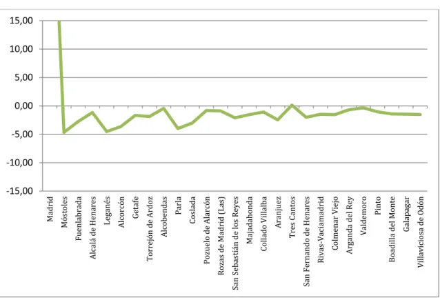
Figure 3a. 𝜹_∙𝒋 coefficients for Madrid province

-15,00 -10,00 -5,00 0,00 5,00 10,00 15,00

Madrid Móstoles Fuenlabrada Alcalá de Henares Leganés Alcorcón Getafe Torrejón de Ardoz Alcobendas Parla Coslada Pozuelo de Alarcón Rozas de Madrid (Las) San Sebastián de los Reyes Majadahonda Collado Villalba Aranjuez Tres Cantos San Fernando de Henares Rivas-Vaciamadrid Colmenar Viejo Arganda del Rey Valdemoro Pinto Boadilla del Monte Galapagar Villaviciosa de Odón

21

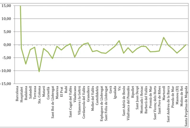
Figure 3b. 𝜹_∙𝒋 coefficients for Barcelona province

Figures 3a and 3b show some common pattern between the two provinces and other results that are more specific. Something common to both cases is that the big cities are the municipalities that can be by far classified as much more capable of attracting new jobs (not surprisingly according to the results already presented in figures 2a and 2b) than new residents. As expected, new workers coming to live in these two provinces have their homes in smaller cities in the surroundings of the capital (those characterized by negative

indicators), but their jobs are located in the urban agglomeration of these two big cities.

In spite of this general picture for both provinces, it is also true that the above pattern is clearer for the case of Madrid than for the case of Barcelona. In this last case, we detect more cases of municipalities (Vic and

example) that could be classified as net receiver of jobs (even when the quantitative difference in the

indicators is still huge). Probably the differences in the industry specialization between these two provinces help to explain such a result: the comparatively larger share of manufacturing companies in the

-15,00 -10,00 -5,00 0,00 5,00 10,00 15,00

Barcelona Hospitalet Badalona Sabadell Terrassa Sta. Coloma Mataró Cornellà Sant Boi de Llobregat Manresa El Prat Rubí Sant Cugat del Vallès Viladecans Vilanova i la Geltrú Cerdanyola del Vallès Granollers Mollet del Vallès Castelldefels Esplugues de Llobregat Sant Feliu de Llobregat Gavà Igualada Vic

Sant Adrià de Besòs Vilafranca del Penedès Ripollet Sant Joan Despí Montcada i Reixac Barberà del Vallès Premià de Mar Sant Vicenç dels Horts Sant Pere de Ribes Martorell Sant Andreu de la Barca Pineda de Mar Masnou (El) Molins de Rei Santa Perpètua de Mogoda

22 province Barcelona, which are located in this type of middle-size cities, is the key factor that accounts for this difference between both cases.

5. Some conclusions

Spain has experienced over the last two decades an intense arrival of immigrants and in-migrants to its central regions. The arrival of population has effects on the recipient regions through internal migrations and/or commuting to some areas that might be more attractive.

Using and extending the input-output model suggested on Fernández-Vázquez

the effects that the arrival of new workers have in the most populated Spanish provinces. Using the last available Census, estimations show that the arrival of in- and im-migration to Madrid and Barcelona generates a set of direct and indirect effects induced by the redistribution of population among other regions.

The arrival of workers provokes reallocations of residence. However, the intensity of these reallocations seems to be correlated with size, which indicates the existence of agglomeration diseconomies associated with big cities. At the same time, when the possibility of commuting is considered the arrival of workers generates both the reallocation of jobs (economic activity) and also of residences. The larger municipalities are the ones pushing out more residents to other areas while keeping most of the jobs. In other words, they are becoming attractive areas to work in (economies of agglomeration), but not to live in (high housing costs, congestion or some other negative externalities).

The opposite is true for the smaller cities, which are resident-absorbing but not job-attracting. Thus, the distribution pattern of residences proves to be different to the distribution pattern of jobs.

Even more, these results highlight the idea that the effects of the arrival of

population are not only felt in the recipient city but might also generate

comparatively far larger effects on other cities in terms of internal migration and

the location of economic activity.

23

Altonji, J. G. and Card, D., 1991. The effect of immigration on the labour market outcomes of less skilled natives, in (J. M. Abowd and R. B. Freeman eds.)

Press.

Angrist, J. D. and Kugler, A. D., 2003. Productive or counterproductive? Labour market institutions and the effect of immigration on EU natives, The Economic

Batty, M., 1983. Linear urban models. Papers in Regional Science, 53, pp. 1-25.

Borjas, G. J., 1997. The economic analysis of immigration, in (O. Ashenfelter and D. Card, eds.), Handbook of Labour Economics, vol. 3A, New York: North Holland.

Card, D. E. and DiNardo, J. E., 2000. Do immigrant inflows lead to native outflows?, American Economic Review, vol. 90 (May), pp. 360–73.

Dietzenbacher, E., 1997. In vindication of the Gosh model: a reinterpretation as a price model, Journal of Regional Science, 37, pp. 629-651.

Fernández-Vázquez, E.; Garcia-Muñiz, A.S. and Ramos-Carvajal C., 2010. The impact of immigration on interregional migrations: an input-output analysis with an application for Spain; Annals of Regional Science, En46 (1): 189-204.

Filer, R. K.,1992. The impact of immigrant arrivals on migratory patterns of native workers, in (G. J. Borjas and R. B. Freeman, eds.) Immigration and the

Chicago: University of Chicago Press.

Frey, W., 1995. Immigration and internal migration "flight" from US metropolitan

areas: toward a new demographic balkanization. Urban Studies, 32, pp. 733-

757.

24 Frey W. H., Liaw, K. L., Xie, Y. and Carlson, M. J., 1996. Interstate migration of the US poverty population: Immigration “pushes” and welfare magnet “pulls”,

Garin. R. A., 1966. A matrix formulation of the Lowry model for intra- metropolitan activity location, Journal of the American Institute of Planners, 32, pp. 361-364.

Guldman, J. M. and Wang, F., 1998. Population and employment density function revisited: a spatial interaction approach. Papers in Regional Science, 77 (2), pp. 189-211.

Hatton, T. J. and Tani M., 2005. Immigration and inter-regional migration in the UK, 1982-2000, The Economic Journal, vol. 115 (November), pp. 342-358.

Jun. M. J., 2005. Forecasting urban land-use demand using a metropolitan input-output model, Environment and Planning A, 37, pp. 1311-1328.

INE, 2007, Censo de Población y Viviendas, 2001, Instituto Nacional de Estadística, Madrid (available online at www.ine.es).

Kritz, M. M. and Gurak D. T., 2000. The impact of immigration on the internal migration of natives and immigrants, Demography, 38 (1), pp. 133-45.

Lowry I. S., 1964. A model of metropolis. Rand Corporation, Santa Monica, California.

McGill, S. M., 1997. The Lowry model as an input-output model and its extension to incorporate full intersectoral relations. Regional Studies, 11 (5), pp.

337-354.

Walker, R., Ellis, M. and Barf, M., 1992. Linked migration systems: immigration

and internal labor flows in the United States, Economic Geography 68, pp. 234-

248.

25 Winter-Ebmer R. and Zweimüller J., 1999. Do immigrants displace young native workers? The Austrian experience, Journal of Population Economics 12, pp.

327-340.

Wright, R., Ellis, M. and Reibel, M., 1996. The linkage between immigration and

internal migration in large metropolitan areas in the United States, Economic

F

C

A

Últimos números publicados

159/2000 Participación privada en la construcción y explotación de carreteras de peaje Ginés de Rus, Manuel Romero y Lourdes Trujillo

160/2000 Errores y posibles soluciones en la aplicación del Value at Risk Mariano González Sánchez

161/2000 Tax neutrality on saving assets. The spahish case before and after the tax reform Cristina Ruza y de Paz-Curbera

162/2000 Private rates of return to human capital in Spain: new evidence F. Barceinas, J. Oliver-Alonso, J.L. Raymond y J.L. Roig-Sabaté 163/2000 El control interno del riesgo. Una propuesta de sistema de límites

riesgo neutral

Mariano González Sánchez

164/2001 La evolución de las políticas de gasto de las Administraciones Públicas en los años 90 Alfonso Utrilla de la Hoz y Carmen Pérez Esparrells

165/2001 Bank cost efficiency and output specification Emili Tortosa-Ausina

166/2001 Recent trends in Spanish income distribution: A robust picture of falling income inequality Josep Oliver-Alonso, Xavier Ramos y José Luis Raymond-Bara

167/2001 Efectos redistributivos y sobre el bienestar social del tratamiento de las cargas familiares en el nuevo IRPF

Nuria Badenes Plá, Julio López Laborda, Jorge Onrubia Fernández

168/2001 The Effects of Bank Debt on Financial Structure of Small and Medium Firms in some Euro- pean Countries

Mónica Melle-Hernández

169/2001 La política de cohesión de la UE ampliada: la perspectiva de España Ismael Sanz Labrador

170/2002 Riesgo de liquidez de Mercado Mariano González Sánchez

171/2002 Los costes de administración para el afiliado en los sistemas de pensiones basados en cuentas de capitalización individual: medida y comparación internacional.

José Enrique Devesa Carpio, Rosa Rodríguez Barrera, Carlos Vidal Meliá

172/2002 La encuesta continua de presupuestos familiares (1985-1996): descripción, representatividad y propuestas de metodología para la explotación de la información de los ingresos y el gasto.

Llorenc Pou, Joaquín Alegre

173/2002 Modelos paramétricos y no paramétricos en problemas de concesión de tarjetas de credito.

Rosa Puertas, María Bonilla, Ignacio Olmeda

174/2002 Mercado único, comercio intra-industrial y costes de ajuste en las manufacturas españolas.

José Vicente Blanes Cristóbal

175/2003 La Administración tributaria en España. Un análisis de la gestión a través de los ingresos y de los gastos.

Juan de Dios Jiménez Aguilera, Pedro Enrique Barrilao González 176/2003 The Falling Share of Cash Payments in Spain.

Santiago Carbó Valverde, Rafael López del Paso, David B. Humphrey Publicado en “Moneda y Crédito” nº 217, pags. 167-189.

177/2003 Effects of ATMs and Electronic Payments on Banking Costs: The Spanish Case.

Santiago Carbó Valverde, Rafael López del Paso, David B. Humphrey

178/2003 Factors explaining the interest margin in the banking sectors of the European Union.

Joaquín Maudos y Juan Fernández Guevara

179/2003 Los planes de stock options para directivos y consejeros y su valoración por el mercado de valores en España.

Mónica Melle Hernández

180/2003 Ownership and Performance in Europe and US Banking – A comparison of Commercial, Co- operative & Savings Banks.

Yener Altunbas, Santiago Carbó y Phil Molyneux

181/2003 The Euro effect on the integration of the European stock markets.

Mónica Melle Hernández

182/2004 In search of complementarity in the innovation strategy: international R&D and external knowledge acquisition.

Bruno Cassiman, Reinhilde Veugelers

183/2004 Fijación de precios en el sector público: una aplicación para el servicio municipal de sumi- nistro de agua.

Mª Ángeles García Valiñas

184/2004 Estimación de la economía sumergida es España: un modelo estructural de variables latentes.

Ángel Alañón Pardo, Miguel Gómez de Antonio

185/2004 Causas políticas y consecuencias sociales de la corrupción.

Joan Oriol Prats Cabrera

186/2004 Loan bankers’ decisions and sensitivity to the audit report using the belief revision model.

Andrés Guiral Contreras and José A. Gonzalo Angulo

187/2004 El modelo de Black, Derman y Toy en la práctica. Aplicación al mercado español.

Marta Tolentino García-Abadillo y Antonio Díaz Pérez 188/2004 Does market competition ma