SALMON (ONCORHYNCHUS TSHAWYTSCHA) IN THE CREDIT RIVER, ONTARIO
Michael Berends
A thesis submitted in conformity with the requirements for the degree of Master of Science,
Graduate Department of Zoology, University of Toronto
© Copyright by Michael Berends (2004)
ivi
of Canada du Canada Acquisitions andBibliographic Services
395 Wellington Street Ottawa ON K1A ON4
Canada Canada
The author has granted a non- exclusive licence allowing the National Library of Canada to reproduce, loan, distribute or sell copies of this thesis in microform, paper or electronic formats.
The author retains ownership of the copyright in this thesis. Neither the thesis nor substantial extracts from it may be printed or otherwise
reproduced without the author's permission.
Acquisisitons et
services bibliographiques
395, rue Wellington Ottawa ON K1A ON4
Your file Votre référence ISBN: 0-612-91584-0 Our file Notre référence ISBN: 0-612-91584-0
L'auteur a accordé une licence non exclusive permettant a la
Bibliotheque nationale du Canada de reproduire, préter, distribuer ou
vendre des copies de cette these sous la forme de microfiche/film, de
reproduction sur papier ou sur format électronique.
L'auteur conserve la propriete du droit d'auteur qui protege cette thése.
Ni la these ni des extraits substantiels de celle-ci ne doivent étre imprimés ou aturement reproduits sans son autorisation.
In compliance with the Canadian Privacy Act some supporting forms may have been removed from this dissertation.
While these forms may be included in the document page count,
their removal does not represent any loss of content from the dissertation.
Canada
i+iConformément a la loi canadienne sur la protection de la vie privée, quelques formulaires secondaires ont été enlevés de ce manuscrit.
Bien que ces formulaires
aient inclus dans la pagination,
il n'y aura aucun contenu manquant.
Michael Berends for the degree of Master of Science, 2003, Graduate Department of Zoology, University of Toronto, Toronto, Canada
Lake Ontario contains both hatchery- and wild-origin chinook salmon (Oncorhynchus tshawytscha), however, researchers do not know the relative proportions and do not have a technique to identify origin. This thesis provides an origin-determination technique based on scale analysis and identifies proportions of hatchery and wild adult chinook in the Credit River. Analysis revealed that the 3-axes method provided a discriminant function with the highest classification level (85.7% with a jackknife cross-validation of 81%). The
discriminant function was developed based solely on differences of scale characteristics
between hatchery and wild fish. Specifically, the characteristics that were utilized were:
focus, STD 3-6, circuli 1, circuli 5, and circuli 2-4.. Using this discriminant function, 58%-
74% of spawning adults in the Credit River were determined to be of wild origin. Thus, we now have an assessment technique and first scientific calculation of the proportion of wild chinook salmon.
ii
Page number (1) Abstract
(D Table of contents
(UD) List of figures and tables (V) Acknowledgements (V) Thesis preface
CHAPTER 1
“A Scale Technique For Identifying Hatchery- And Wild-Origin Chinook Salmon”
Introduction
Ringwood Hatchery
Wilmot Creek
Methods
Scale and image preparation
Image analysis and measurement of scales Axes groups
Hatchery and wild Groups Scale pattern measurements Data analysis
Discriminant function analysis Results
Mean circuli width
Standard deviation of circuli width (STD) Axes choice
Variable comparison between hatchery and wild scales Discriminant function analysis
Discriminant function analysis by axes-group Discussion
Axes comparison
Growth patterns Discriminant functionImplications
li
il iii
vi viii
In HKD uw BW
10
10
il
11
il
12
12
15
17
18
22
23
26
26
26
27
28
References
CHAPTER 2
“Hatchery- And Wild-Origin Chinook Salmon In The Credit River, Ontario”
Introduction
History of chinook salmon stocking in Lake Ontario Chinook salmon biology
Chinook growth and age Chinook production in Lake Ontario
Broodstock origin
Hatchery production in Lake Ontario Wild production in Lake Ontario Credit River
History and physiography
Chinook in the Credit River
Wild production in the Credit River Hatchery vs. wild Survivorship
Introduced species
Great Lakes biodiversity Theory
Hatcheries Credit River
Hypothesis, Predictions and Tests
HypothesisPrediction #1
Test of prediction #1
Prediction #2Test of prediction #2 Methods
Study site
iv
32
35
36 36 39 40 40 41 42 43 4]
47 50 52 53 53 54 57 57 58 60
60
60
60
60
61
61
61
Credit River Scale analysis
Scale and image preparation
Image analysis and measurement of scales Discriminant function analysis
Phenotype analysis Statistical analysis
Results
Origin identification Phenotype analysis Discussion
Run-time
Limitations of data
Management and conservation implications Applications
Hatcheries Future studies
Emergence of a wild run
SummaryReferences
62
65
65
65
66
67
68
68
68
70
76
78
78
79
82
82
83
83
84
85
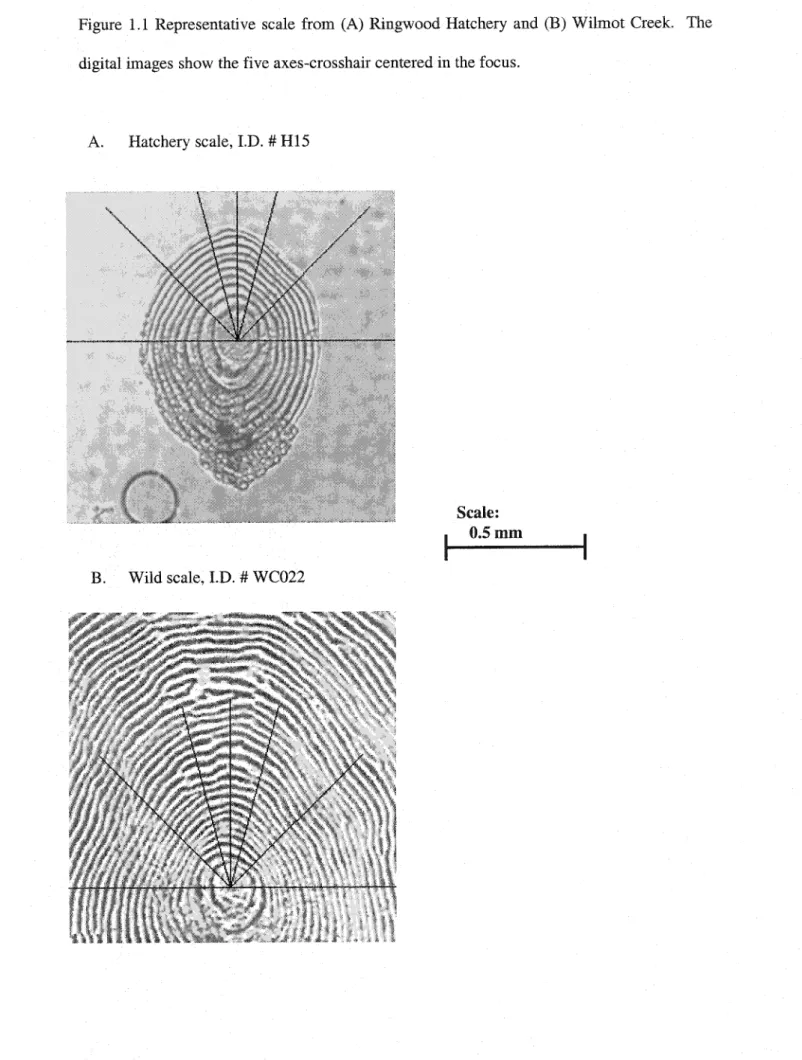
Figure 1.1 Representative scale from Ringwood Hatchery and Wilmot Creek.
Table 1.1
Table 1.2
Table 1.3
Table 1.4
Table 1.54
Table 1.5B
Table 1.5C
Table 1.6
Table 1.7
Figure 2.1
Circuli width for hatchery and wild-produced chinook salmon measured
with l-axis, 3-axes and 5-axes.
Standard deviation of circuli width for hatchery and wild-produced chinook salmon measured with 1-axis, 3-axes and 5-axes.
Comparison of focus area (mm”), individual circuli widths (mm), and mean cumulative circuli width (mm) of the first 6 circuli of hatchery and wild chinook, using the 3-axes group.
Standard deviation of circuli width (mm) for hatchery and wild-produced chinook salmon measured with the 3-axes group.
Classification summary and cross-validation of the discriminant function
Non-standardized (Raw) and standardized relative weights of predictor
variables for the linear discriminant function.
Discriminant functions with one variable removed from the discriminant function (85.7 %) and classification levels for discriminant functions
developed with individual variables.
Classification summary and cross-validation of the 1-axis discriminant function.
Classification summary and cross-validation of the 5-axes discriminant function
The Credit River and other major tributaries of Lake Ontario.
vi
14
16
20
21
24
24
24
25
25
38
in Lake Ontario.
Figure 2.2B Number of wild chinook and coho salmon juveniles observed during summer electrofishing surveys of Lake Ontario tributaries in Ontario.
Figure 2.3. Map of the Credit River.
Figure 2.4 History of chinook salmon stocking in the Credit River, Ontario.
Table 2.1 “Introduced species” of fish have entered the Great Lakes by a variety of vectors:
Figure 2.5 Collection times of adult chinook salmon from the Credit River 2001.
Table 2.2 Credit River origin identification probability -level summary.
Table 2.3. Sex ratios for each confidence level.
Table 2.4 Fork length, body weight and kype length for females at each classification level
Table 2.5 Fork length, body weight, and kype-length for males (minus jacks) at each classification level.
Table 2.6 Fork length and body weight for male jacks at each classification level.
Table 2.7 Comparison of run-time between hatchery and wild adult chinook from
the Credit River
vil
45
46
49
31
56
64
69
73
73
74
74
75
I am grateful to my supervisor Dr. Mart Gross for his encouragement, advice, and guidance throughout the course of this work. I thank him for his thesis revisions, financial support for 2 years, and use of research support facilities. His enthusiasm and passion for conservation biology and his thirst for knowledge have been a great example to me.
I also thank my committee member Dr. Brian Shuter for his assistance in the development and review of my thesis and Dr. Joe Repka, Professor of mathematics, for his
advice and guidance.
Several members of the Ontario Ministry of Natural Resources (OMNR) were extremely helpful at various stages of this research. In particular, I thank Jim Bowlby, Les Stanfield, Lisa Miller-Dodd, and Tom Stewart.
I had the fortunate experience of sharing the lab with some great graduate student and even better friends, Karin von Ompteda, Ian Craine, and Cory Robertson. Their intellectual
support and friendship are very much appreciated. Many great times were shared between us and I will always cherish them. An additional thank you to all of the people who assisted with the field data collection and with the lab analysis, particularly, Johnston Miller, and
Alexandra Smith.
Though there were many people who helped along the way, a special thanks goes to Darren Batt. His willingness to help had no boundaries. From jumping in a cold river, moving freezers, cutting up dead fish, to lending a “little” financial support, he was always there for me, thank you.
Finally, thank you to my mom and dad who have supported my efforts in science with enduring loyalty. A loving thank you to for allowing me to chose my own path and always supporting me, I know it wasn’t always easy. Your encouragement and enthusiasm have always been deeply felt. Iam forever indebted.
vill
separated us, you have always been by my side. Your encouragement, support, and love has made it possible for me to be where I am today. I dedicate this thesis to my parents and Cecile.
ix
This thesis contains two chapters. The first “A scale technique for identifying
hatchery and wild chinook salmon’, provides a technique for identifying whether chinook
salmon natal origin is from a hatchery or the wild. The second chapter, “Hatchery- and wild-
origin chinook salmon in the Credit River, Ontario”, applies the developed technique to
determine the relative proportions of hatchery and wild origin of spawning adults. It also compares some aspects of their phenotypes. Both chapters are prepared with their own Introduction, Methods, Results, Discussion, Conclusion, and References.“A Scale Technique For Identifying Hatchery- And Wild-Origin Chinook
Salmon”
Lake Ontario chinook salmon (Oncorhynchus tshawytscha) are produced by both
hatcheries and wild spawning (Kocik and Jones 1999). Although fisheries managers wish to regulate their total abundance, to date there has been no technique developed to identify theorigin of chinook in Lake Ontario. As such, managers are unable to properly estimate the relative contributions of hatchery and wild production to the fishery.
A commonly used method for the identification of chinook stocks in their native range is scale pattern analysis (SPA) (Myers et al. 1987). After attempting this with Lake Michigan chinook salmon, Carl (1982) concluded that “Annual differences in growth indicated discriminant analysis or other mixing problem solutions applied to scale measure data from
adults would be of very limited usefulness in determining the contribution of wild fish to the
Lake Michigan fishery”.The purpose of this paper is to: (1) illustrate how multiple axes improve resolving power and the capacity to differentiate Lake Ontario chinook salmon of hatchery and wild
origin; (2) characterize differences in early growth experienced by hatchery- and wild-origin
chinook; and, (3) provide a discriminant function with the capacity to identify hatchery- and wild-origin fish.In many species of fish, including Pacific salmon, the use of scale analysis as a tool
for stock identification depends on a high correlation between the nature of a fish’s growth
and the pattern in the fish’s scale (Koo 1955; Clutter and Whitesel 1956). Salmon emergefrom their egg without scales. As the fish grows, rudimentary scales develop that under
magnification, display numerous concentric rings called circuli radiating outward from a central focal area (Schwartzberg and Fryer 1993). Fish and scale growth are influenced by environmental conditions such as food availability, water temperature, length of growingseason, and may also be influenced by genetic factors (Schwartzberg and Fryer 1993). Once
growth of the scale width. However, formation of circuli is not at fixed size intervals, as it is
related to both time and growth (Bilton 1975).
Stock identification based on scale analysis is possible when scale pattern differences
found between groups or stocks are greater than among individuals within a stock. Hatchery- reared salmon generally grow faster than those produced in the wild and their growth is generally more uniform (Peck 1970). The increased and more consistent growth characteristics of hatchery than wild fish can appear in the spacing of circuli and allow for thediscrimination of the two groups (Stokesbury e¢ al. 2001). Furthermore, focus area has been
shown to be a useful variable for discerning wild and hatchery-produced fish. Stokesbury et al. (2001) found focus area to be smaller in wild-produced Atlantic salmon (Salmon salar) (25 mm” focus area) than in farm-produced salmon (28 mm’). This result was attributed to the size difference between the two groups of fish at platelet formation. That is, the size ofthe focus would be proportionally bigger in fish of hatchery origin than of wild origin due to
larger egg size and better developmental conditions for those in the hatchery.Fisher (1936) introduced the discriminant function as a method of classifying individuals from mixed samples into their natal groups. Linear discriminant analysis permits the simultaneous use of independent variables to form classification functions that identify
groups. In this method, a set of measurements from an individual is reduced to a single value by which the individual is classified as being from one group or the other. This methodology
has been applied and proven useful in determining the origin of individual salmon stocks from scales in mixed-stock samples (Unwin and Lucas 1993, Stokesbury et al. 2001).Wild production raises a suite of concerns for the Lake Ontario ecosystem including:
(1) potential impacts on native species (e.g., brook trout (Salvelinus fontinalis)); (2) impacts on other stocked species (brown trout (Salmo trutta) and rainbow trout (Oncorhynchus
collapse of the food web (e.g. alewife (Alosa pseudoharengus)) and thus the fishery; and, (5)
the transfer of contaminants into the lake watershed. Since the complete control of chinook
production by managing hatcheries may no longer be possible, and because the full ecological implications of this non-indigenous species in the Lake Ontario ecosystem are unknown, it is essential that a better understanding of both hatchery and wild populations beobtained. To help achieve this early growth patterns from both hatchery and wild-produced individuals collected from the Ringwood Hatchery and from Wilmot Creek in the Lake
Ontario watershed, respectively were analyzed.Ringwood Hatchery
Influenced by the groundwater temperature (8°C) at the Ringwood Hatchery (Mount Albert, Ontario), the chinook begin hatching in early December. External feeding begins during the 2nd —3rd week of January (defined as month one, when there is 100% hatch in the lot) and continues daily until two days before stocking. The fish are fed ad libitum and food is incremented on a daily basis to maximize growth. This contrasts with most other OMNR
(Ontario Ministry of Natural Resources) hatchery-raised species that have their feed increased only on a weekly basis or less often (L. Miller-Dodd, OMNR, pers. com. Feb 1, 2002).
Juvenile hatchery fish (4-6g) are stocked into Lake Ontario and its tributaries during
the last few weeks of April and sometimes early May but no later than May 10th, by which time the receiving waters are usually too warm in comparison to the rearing temperature.
Hatchery fish stocked into river systems are mot seen in the river afer rani-viay. Most fish
leave the river following the first major rainfall! after stocking, which can occur after a few days to a few weeks (J. Bowlby, OMNR, pers. com. Fume 15, 2001). The juveniles are estimated to weigh 5 to 10 grams (70-100 mm FL) at the time of entry to the Iske. However,4
annually.
The Credit River spawning run consists of adult chinook that are believed to be
mainly 2 and 3-years old (Schaner et al. 2001). Two-year old fish are those that are new juveniles in spring and return in fall two calendar years later (e.g. released spring 1998 and
return fall 2000; in fall 1998 they are still age 0, fall 1999 is age 1, fall 2000 is age 2 and fall 2001 is age 3). Adult chinook begin their entry into the Credit River in late August or early September, depending on water level conditions, and continue to enter through October.Each year OMNR collects approximately 400 (1:1 sex ratio) returning adults during the first two weeks of October. Gametes are stripped and returned to the Ringwood Hatchery where crosses are made and embryos and alevins are reared (L. Miller-Dodd, OMNR, pers. comm.
Sept 19, 2003). Finally, hatchery juveniles are stocked back into the Credit River and other locations throughout the lake during April/May. Approximately 100,000 to 150,000
hatchery-produced juveniles are released annually into the Credit River.
Wilmot Creek
Wilmot Creek is a tributary of Lake Ontario located 80 km east of Toronto. It is believed that the adult spawning run of chinook in Wilmot Creek consists of wild fish (99%
or more, J. Bowlby, OMNR, pers. com. August 8, 2003). This assumption is based on two important features of the river: (1) the high natural production of chinook fry each spring (225,000 estimated in May 2002, I. Craine, pers. com. Aug, 20, 2003); and (2) the lack of
hatchery stocking.
Approximately 90% of wild juveniles are estimated to outmigrate in the year of their emergence from late May through mid-June (Bowlby ef al. 1998). This would correspond to the ocean-type life history typical of Washington State chinook salmon (Healey, 1998). Wild
mm) than hatchery smolts during lake entry. Thus, wild fish have a shorter growth period before lake-entry, as compared to hatchery fish who emerge in January.
In the present thesis I show that by measuring scale circuli and analyzing early growth patterns via multiple axes, it is possible to develop a discriminant function that differentiates
hatchery and wild-produced chinook salmon in Lake Ontario.
Methods
Scale and image preparation
Scales were collected from the preferred area for chinook, which is below the
posterior edge of the dorsal fin and 2-4 scale rows above the lateral line on the left side
(Schwartzberg and Fryer 1993). The area was cleaned of mucus and dirt, and scales weresampled by pulling individual scales with forceps and placing them directly into labeled
containers. Since it was difficult to determine the quality of scales during their removal, a larger sample of 10-15 scales was taken from each individual.The scales (~ 4-5) were later mounted on glass slides with 60% glycerol under cover- slips flattened and sealed with nail polish. Two to four scales from each fish were examined using 2 compound microscope (Olympus CK2). The scales were magnified 40X, resulting in a resolution of 341 pixels per inch and a digital file size of 513 KB per scale. Images were
made with a digital camera (COHU — high performance CCD camera) connected to a
compound microscope and saved on the computer using Optimas software (Optimas 5.1, 1995). Files were saved as 8-bit grayscale “.tif” files. Image files were then transferred to Fireworks software (Fireworks 4, 2002) and transformed to provide an image with a higher number of pixels. The transformation procedure was: (1) crop to 640X480; (2) resize canvas size to 800X800; (3) rotate image as needed; (4) re-crop image to 300X300; (4) modifyimage resolution, not image calibration). Changing the resolution simply increases the
number of pixels on the image (pixel density), resulting in approximately 100-120 pixels in-
between each circuli as compared to 8-12, the number prior to the resolution increase. This
change was important since the software measuring tool is limited to measuring pixels. The
software is coded to know the size of pixels and uses pixels as the element of measurement;
(5) place “crosshair” (see below) onto center of focus, located by eye; and (6) save file (size =
25,000 KB). The increase in resolution resulted in a calibration of 1 pixel being equal to
0.00022 mm in length.Image analysis and measurement of scales
Bersoft image measurement software (Bersoft, 2002) was used to evaluate the scales.
Traditional scale analysis is done with linear measurements taken along a line perpendicular to a reference line as described in Schwartzberg and Fryer (1993). However, for the purpose
of reducing the “noise” of irregularities along circuli, we decided to use multiple linearmeasurements. A “crosshair” was placed in the center of the focus, consisting of a
perpendicular line, 2 lines 15° degrees from the perpendicular line, and 2 lines 45° degrees oneither side of the perpendicular line (Figure 1.1). The crosshair was centered with the perpendicular line passing through the focus close to, or on, the longest axis of the scale;
some latitude was given to adjust for the effects of strong asymmetry of some scales. On average, hatchery juveniles had 8 (minimum 6) circuli and the adults had approximately 30.
Hatchery juveniles were limited in the number of their circuli due to their amount of growth at time of collection, whereas, at the same magnification, the number of circuli seen on adult scales was only limited by the size of the image.
mm along the axes on each scale. Circulus width was measured as the distance from the end of one circulus to the end of the next circulus. In addition, the periphery of the focal area was traced and area measurements (mm”) of scale foci were calculated by the “area measurement tool” (Bersoft, 2002).
Figure 1.1 Representative scale from (A) Ringwood Hatchery and (B) Wilmot Creek. The digital images show the five axes-crosshair centered in the focus.
A. Hatchery scale, 1D. # H15
Scale:
0.5 mm |
B. Wild scale, LD. # WC022
Axes groups
The purpose of the additional axes above the single axis usually applied in scale analysis (e.g. Schwartzberg and Fryer 1993) was to test for the incremental value in characterizing growth patterns with more data. Thus, measurements of circuli along the
“crosshair” were divided into three groups: (1) 1-axis, consisting of measurements made along the traditional axis that runs vertically through the middle of the scale; (2) 3-axes,
consisting of the main-axis plus the two additional axes that were 15° degrees from the main
line; and (3) 5-axes, consisting of the main-axis, the two axes 15° degrees from the main line,and 2 additional axes 45° degrees on either side of the main line. Since circuli are laid down
on the scale in a concentric manner and radiate outward from a central focal area (Schwartzberg and Fryer 1993), the measured distance between circuli depends on the angle of measurement. Thus, on average, the main-axis has the greatest separation between circuli.This separation decreases as one moves away on either side of the main line and, as axes are added away from the center, the average distance between circuli decreases.
Hatchery and Wild Groups
Juveniles (n = 20) were received at the Ringwood Hatchery from the OMNR on May 10 2002, during the annual stocking of the Credit River (fish were euthanised with MS-222).
These hatchery fish have similar scale growth to those that are released each year since the hatchery rears the fish annually in the same manner and with the same duration. Scales were removed from hatchery fish for scale analysis.
It was not possible to retrieve scales from wild juveniles due to the extremely small size of the scales and difficulty of removing them without damage. Therefore, scales were taken from 22 adult chinook from Wilmot Creek collected from the 29" Sept to 25%
November 2002 by Ian Craine (Gross Lab, University of Toronto).
Scale pattern measurements
The four categories of patterns measured were: (1) Width of individual circuli,
measured from the end of a circulus to the end of the next circulus (e.g. end of focus to the
end of circulus 1 = circulus 1, circulus 1-circulus 2 = circulus 2, ... circulus 5-ciruclus 6 =
circulus 5); (2) Mean width of the first 6 circuli [(circulus 1+ circulus 2...circulus 6)/6] and mean width of circuli 2-4 (i.e. circuli 1-6 and 2-4 are the summations of the individual circuli
widths for the first six circuli and the second through fourth circuli respectively); (3) Standard deviation of the width of pairs of circuli as well as inclusive combinations (i.e. STD- 1-6, 2-
6, 3-6, 4-6, 5-6, 1-2, 3-4, 3-5, 4-5). STD is the absolute difference in circuli width between
consecutive circuli; and (4) Area of the focus (mm’).
Two scales from each fish were analyzed and the mean measurements of the two scales were used in the analysis (paired t-tests on the difference between the two measurements from the same individual revealed that they were not significantly different, e.g. focus, P = 0.72).
Data analysis
A series of t-tests were performed on the scale measured derived variables of the hatchery and wild groups using the Minitab statistical software package (Release 11.21, 1996). Comparison of the two control groups was made using measurements up to the first 6 circuli, since 6 was the minimum number of circuli (growth) that each individual from the hatchery had at the time of collection. Statistically significant results were those that had p- values less than 0.05 (the generally accepted level for biologists). However, results were also
_ tested at the 0.01 level to test for the strength of the results.
Discriminant function analysis
Discriminant analysis is a method of linear modeling that proceeds in two steps.
Specifically, one first tests for differences in the explanatory variables among predefined groups (e.g. t-tests). If the test supports significantly different variables between groups, one then proceeds to find the linear combinations (called discriminant functions or identification functions) of the variables that best discriminate among the groups (Legendre and Legendre,
1998).
For this study, all variables that were significant (p<0.05, two-tailed t-test analysis) predictors of origin were tested in the development of the function. A stepwise procedure was applied in the analysis, allowing variables to be entered or removed from a discriminant function at each stage of function development. This procedure resulted in a linear discriminant function that maximized the difference between the two control groups.
The discriminant function was then tested with a jackknife cross-validation procedure (Legendre and Legendre, 1998). This technique is used to compensate for an optimistic
apparent error rate (AER), defined as the number of misclassified observations in the data set
divided by the total number of observations in the data set. AER tends to be optimistic because the data being classified are the same data used to build the classification function.This procedure omits the first observation from the data set, develops a classification function using the remaining observations, and then classifies the omitted observation. Next, it returns
the first observation to the data set, omits the second observation, repeats the same process, and continues in this manner with all observations in the data set.
Results
Mean circuli width
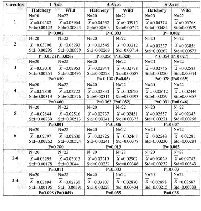
Significant differences were found between hatchery- and wild-produced circuli with
each of the 1-, 3-, and 5-axes groups (Table 1.1). However, the axes groups differed in the
total number of significantly different individual circuli. With the l-axis group there were only two significantly different circuli (circuli- F-1 and 4-5), whereas with the 3- and 5-axes
groups there were three significantly different circuli between hatchery and wild fish (circuli- 1, 5, and 6). In addition, when analyzing combinations of circuli, the 1-axis only had meancirculi 1-6 significantly different, while the 3- and 5-axes groups had both mean circuli 1-6 and mean circuli 2-4. Therefore, the 3- and 5-axes groups include all of the significant circuli found with the 1l-axis, plus an additional significantly different circuli (circuli 6), and an
additional significantly different mean circuli width(circuli 2-4).Both the 3- and 5-axes groups resulted in the same four significantly different circuli at the 0.05 probability level (circuli-i, 2, 5, and 6). At a level of 0.01, both have three
significantly different circuli, although with some difference (3-axes: circuli-1, 2, and 5; 5- axes: circuli-1, 5, and 6). For the 3-axes the circuli were 1, 2, and 5, whereas for the 5-axes the circuli were 1, 5 and 6.
All the above t-tests were 2-tailed t-tests and thus were conservative tests since they were not assessed using a prediction of growth differences (i.e. hatchery fish have greater growth, e.g. Stokesbury et al. 2001). If this prediction is accepted, than it is valid to compare the variables using 1-tailed t-tests. When such tests are performed, the 2-tailed p-value is divided by “two”, and all of the circuli widths in the 3-axes and 5-axes between the two
groups are found to be significant (i.e. circuli 2, 3, and 4 are all p <0.05). In addition, circuli
2, and 2-4 become significant when using the main-axis (Table 1.1).Furthermore, in regards to tables 1.1-1.3 and the statistical issue of multiple statistical
tests, sequential Bonferroni corrections are not needed. This is because, as stated by Moran (2003); (1) the significant results were planned comparisons (i.e. hatchery vs. wild), (2) the results satisfy the rules of logic and reason (there are patterns seen along each axes group);and, (3) there is more than one highly significant result in each table.
Table 1.1 2-tail t-tests of circuli width (mm) for hatchery- and wild-origin chinook salmon measured with l-axis, 3-axes, and 5-axes. Significant P-values are highlighted (N=
number of fish, X = mean circuli width, and Std = standard deviation). i-tailed t-test P- values are in brackets.
Circulus 1-Axis 3-Axes 5-Axes
Hatchery Wild Hatchery Wild Hatchery Wild
N=20 N=22 N=20 N=22 N=20 N=22
1 X =0.04582 X =0.03964 X =0.04532 X =0.03915 X =0.04374 X =0.03768 Std=0.00429 | Std=0.00843 | Std=0.00503 | Std=0.00712 | Std=0.00484 | Std=0.00679
P=0.005 P=0.003 P= 0.002
| N=20 N=22 N=20 N=22 N=20 N=22
2 X =0.03706 | X =0.03293 | X =0.03546 | X =0.03212 | X =0,03337 | X -0.03058
Std=0.00296 | Std=0.00879 | Std=0.00269 | Std=0.00714 | Sid=0.00267 | Std=0.00573 P=0.052 (P=0.026) =0.056 (P=0.028) P=0.054 (P=0.027) N=20 N=22 N=20 N=22 N=20 N=22 3 X =0.03010 X =0.02953 X =0.02944 X =0.02778 X =0.02746 X =0.02583
Std=0.00264 | Std=0.00495 | Std=0.00228 | Std=0.00387 | Std=0.00220 | Std=0.00344
P=0.650 P= 0.100 (P=0.05) P=0.078 (P=0.039)
N=20 N=22 N=20 N=22 N=20 N=22
4 X =0.02830 X =0.02722 X =0.02830 X =0.02620 X =0.02612 | X =0.02444 Std=0.00313 | Std=0.00576 | Std=0.00311 | Std=0.00393 | Std=0.00259 | Std=0.00357
P=0.460 P=0.063 (P=0.032) P=0.091 (P=0.046)
N=20 N=22 N=20 N=22 N=20 N=22
5 X =0.02844 X =0.02516 X =0.02737 X =0.02451 X =0.02557 X =0.02343 Std=0.00239 | Std=0.00513 | Std=0.00241 | Std=0.00373 | Std=0.00221 | Std=0.00266
P=0.001 P=0.006 P=0.007
N=20 N=22 N=20 N=22 N=20 N=22
6 X =0.02797 X =0.02630 X =0.02726 X =0.02468 X =0.02548 X =0.02281 Std=0.00262 | Std=0.00524 | Std=0.00241 | Std=0.00378 | Std=0.00230 | Std=0.00284
P=0.200 P=0.013 P= 0.002
N=20 N=22 N=20 N=22 N=20 N=22
1-6 X =0.03295 | X =0.03013 | X =0.03219 | X =0.02907 | X =0.03029 | X =0.02742
Std=0.00178 | Std=0.0044 Std=0.00237 | Std=0.00386 | Std=0.00232 | Std=0.00343
P=0.011 P=0.003 P=0.003
N=20 N=22 N=20 N=22 N=20 N=22
2-4 X =0.02894 X =0.02730 X =0.03107 X =0.02870 X =0.02898 X =0.02687 Std=0.00196 | Std= 0.00391 | Std=0.00228 | Std=0.00434 { Std=0.00215 | Std=0.00388
P=0.098 (P=0.049) ~ P=0.035 P=0.038
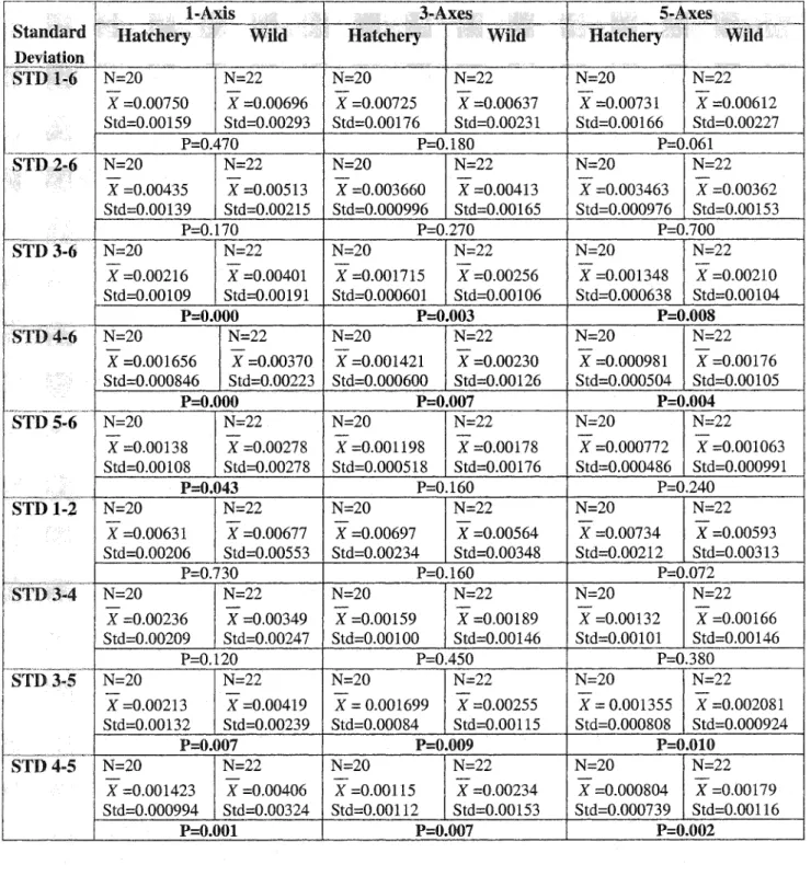
Standard deviation of circuli width (STD)
The STD was defined as: the average deviation from the mean circuli width over a specified range of circuli number and is a measure of the amount of variation in consecutive
ny, (> x)
1
_-="— where n= the n(n —1)
circuli widths. Mathematically it is calculated as: STD=
number of circuli and x = circuli width.
The combinations of circuli measured with the 1-axis provided the greatest number of significantly different STD variables (Table 1.2). The 1-axis showed five STD variables, 3-6,
4-6, 5-6, 3-5, 4-5, to be significant at the 0.05 level and all but STD 5-6 were significant at
the 0.01 level. For the 3-axes, 4 STD variables (3-6, 4-6, STD 3-5 and 4-5) were significant
at both the 0.05 and 0.01 level. The 5-axes showed 4 STD variables, 3-6, 4-6, 3-5, 4-5, to be
significant at both the 0.05 and the 0.01 level. Overall, for each of the axes-groups, theSTD’s from circuli 2 to circuli 6 inclusive were larger in the wild group, whereas the STD of
the first two circuli (1-2) was higher in the hatchery group.Table 1.2. 2- tailed t-tests of standard deviation (STD) of circuli width for hatchery- and wild-origin chinook salmon measured with 1-axis, 3-~axes, and 5-axes. STD defined as: the average deviation from the mean circuli width over a specified range of circuli number and is a measure of the amount of variation in consecutive circuli widths. Significant P-values are highlighted (N= number of fish, X= mean circuli width, and Std = standard deviation).
LAxis 2 | Axes | 5-AXeS
Standard | Hatchery Wild Hatchery Wild Hatchery Wild
Deviation
STD 1-6 | N=20 N=22 N=20 N=22 N=20 N=22
X =0.00750 X =0.00696 | X =0.00725 X =0.00637 X =0.00731 | X =0.00612 Std=0.00159 | Std=0.00293 | Std=0.00176 | Std=0.00231 | Std=0.00166 | Std=0.00227
P=0.470 P=0.180 P=0.061
STD 2-6 | N=20 N=22 N=20 N=22 N=20 N=22
X =0.00435 X =0.00513 | X =0,003660 | X =0.00413 X =0.003463 | X =0.00362 Std=0.00139 | Std=0.00215 | Std=0.000996 | Std=0.00165 | Std=0.000976 | Std=0.00153
P=0.170 P=0.270 P=0.700
STD 3-6 | N=20 © N=22 N=20 N=22 N=20 N=22
X =0.00216 X =0.00401 | ¥ =0.001715 | ¥ =0.00256 X =0.001348 | X =0.00210 Std=0.00109 | Std=0.00191 | Std=0.000601 | Std=0.00106 | Std=0.000638 | Std=0.00104
P=0.000 P=0.003 P=0.008
STD 4-6 | N=20 N=22 N=20 N=22 N=20 N=22
X =0.001656 | X =0.00370 | X =0.001421 | X =0.00230 X =0.000981 | X =0.00176 Std=0.000846 | Std=0.00223 | Std=0.000600 | Std=0.00126 | Std=0.000504 | Std=0.00105
P=0.000 P=0.007 P=0.004
STD 5-6 | N=20 N=22 N=20 N=22 N=20 N=22
X =0.00138 X =0.00278 | X =0.001198 | X =0.00178 X =0.000772 | X =0.001063 Std=0.00108 | Std=0.00278 | Std=0.000518 | Std=0.00176 | Std=0.000486 | Std=0.000991
P=0.043 P=0.160 P=0.240
STD 1-2 | N=20 N=22 N=20 N=22 N=20 N=22
X =0.00631 X =0.00677 | X =0.00697 X =0.00564 X =0.00734 | X =0.00593 Std=0.00206 | Std=0.00553 | Std=0.00234 | Std=0.00348 _| Std=0.00212 | Std=0.00313
P=0.730 P=0.160 P=0.072
STD 3-4 | N=20 N=22 N=20 N=22 N=20 N=22
X =0.00236 X =0.00349 | X =0.00159 X =0.00189 X =0.00132 | X =0.00166 Std=0.00209 | Std=0.00247 | Std=0.00100 | Std=0.00146 _| Std=0.00101__| Std=0.00146
P=0.120 P=0.450 P=0.380
STD 3-5 | N=20 N=22 N=20 N=22 N=20 N=22
X =0.00213 X =0.00419 | X =0.001699 | X =0.00255 X = 0.001355 | X =0.002081 Std=0.00132 | Std=0.00239 | Std=0.00084 | Std=0.00115 _| Std=0.000808 | Std=0.000924
P=0.007 P=0.009 P=0.010
STD 4-5 | N=20 N=22 N=20 N=22 N=20 N=22_
X =0.001423 | X =0.00406 | X =0.00115 X =0.00234 X =0.000804 | xX =0.00179 Std=0.000994 | Std=0.00324 | Std=0.00112 | Std=0.00153 | Std=0.000739 | Std=0.00116
P=0.001 P=0.007 P=0.002
Axes choice
The results of the 2-tailed t-tests performed on circuli width measurements of the
main-, 3-, and 5-axes groups demonstrated that using the 3- and 5-axes identifies more significant difference between the hatchery and wild groups than the l-axis. The 3-axes method is, in total, better to use than the main-axis method when analyzing circuli width since: (1) it had more significant circuli at 0.05 level; and, (2) it incorporated all of the circulithat were significant when using the main-axis group.
However, adding 2 additional axes to the 3-axes, for a total of 5, did not result in a
higher power of resolution. The 3-axes also requires less measurement effort. Specifically, it
is estimated that it takes approximately 5 minutes longer per scale when measuring 3 axes compared to | axis, and an additional 4 minutes when measuring 5 axes compared to 3 axes.Comparing the t-test results of the STD variables when using the main-, 3-, and 5- axes groups suggested the 5-axes with 5 significant characters between the hatchery and wild groups, gave the greatest resolution. However, only one set of measurements composes the standard deviations of the circuli from each scale when using one axis. Such a method allows
“noise” and inherent natural variance due to the single set of measurements. used in development of the width of each circuli. This “noise” is seen in the higher levels of variance in the STD variables of the main-axis than in either of the 5- and 3-axes groups (Table 1.2).
Although the STD variables are larger in the 3-axes than in the 5-axes, the difference is not as great when comparing the main-axis. Both the 5- and 3-axes decrease the level of “noise”
since there is less measurement error due to the “smoothing” of the measurements over 3 and/or 5 axes.
Furthermore, it is important to note that since the variables are to be utilized in the development of a discriminant function, the variables must be independent of one another if more than two are used in the function. Therefore, since several of the variables that were
tested for STD’s are components of one another, not all of the variables can be used
simultaneously during the development of the function. Consequently, the variable that contains the most information on the standard deviations of the circuli growth patterns and is also significant is STD 3-6. This variable has a higher significance level with the 3-axes (p=0.003) than with the 5-axes group (p=0.008), therefore it is concluded that overall (i.e. for
circuli width and standard deviation variables) the 3-axes is the best axis group to use when developing the discriminant function.
Variable comparison between hatchery and wild scales
Scale measurement variables were tested to find those that most effectively characterized differences between hatchery and wild fish. Only results of t-tests on the 3-
axes group are presented since these results provide the superior discriminant function (see below). Table 1.3 provides the results of t-tests between hatchery and wild fish for 3-axes, revealing the significantly different growth rates between the two origin-groups. Results revealed that hatchery-origin chinook relative to wild-origin have a significantly larger focalarea (X = 0.02866" mm vs. X= 0.02468* mm), larger width of each of the first six
consecutive circuli pairs (three significantly different; circuli 1, 5 and 6), a significantly larger
mean width across the first 6 circuli (1-6; X =0.03219 mm vs. X =0.02907 mm), and across
circuli 2-4 (X =0.03107 mm vs. X = 0.02870 mm). Furthermore, the wild group was found to
have larger standard deviations of circuli widths from circuli 2 to circuli 6 inclusive (Table
1.4). Of these variables, 4 were significantly different (STD 3-6, STD 4-6, STD 3-5 and STD 4-5). Due to the opposite trend of STD 1-2 and STD 3-6 between the two origin-groups, thestandard deviation of 1-6 was not significantly different.
Focal area and the spacing of each of the first six circuli were notably larger for hatchery-origin fish than for wild-origin. Analyzing the results of the STD measurements
revealed that the STD for circuli 3-6 was significantly larger for the wild group, and the STD of 1-2 was slightly larger for hatchery fish but this difference was not statistically significant (p=0.16). Thus, when the two STD variables (1-2 and 3-6) were combined the standard deviation of the first six circuli (STD 1-6) was not found to be significantly different.
Overali, this analysis clearly reveals that the two origin-groups are different in their respective patterns of circuli growth. Specifically, scales of hatchery fish show greater and more consistent growth than wild fish.
Table 1.3 Comparison of focus area (mm’), individual circuli widths (mm), and mean cumulative circuli width (mean sum of means in mm) of the first 6 circuli of hatchery- and
wild-origin fish, using the 3-axes group. (N= number of fish, X = mean circuli width, and
Std = standard deviation).
Variable Hatchery Wild
Focus Area N=20 N=24
X =0.02866 | X =0.02468 Std= 0.00343 | Std=0.00601
P=0.014
N=20 N=22
Circulus 1 X =0.04532 | X =0.03915 Std=0.00503 | Std=0.00712
P=0.003
Circulus 2 N=20 N=22
X =0.03546 X =0.03212 Std=0.00269 Std=0.00714
_ P= 0.056
Circulus 3 N=20 N=22
X =0.02944 X =0.02778 Std=0.00228 Std=0.00387
P= 0.100
Circulus 4 N=20 N=22
X =0.02830 X =0.02620 Std=0.00311 Std=0.00393 pe : ae P=0.063
Cireulus 5 N=20 N=22
X =0.02737 X =0.02451 Std=0.00241 Std=0.00373
P=0.006
Circulus..6 N=20 N=22
X =0.02726 X =0.02468 Std=0.00241 Std=0.00378
weansyietie et pi rattan P=0 0 i 3
Mean Circuli N=20 N=22
Width 1-6 X =0.03219 | X =0.02907 Std=0.00237 | Std=0.00386
P=0.003
Mean Circoli N=20 N=22
Width 2-4 X = 0.03107 | X =0.02870 Std= 0.00228 | Std=0.00434
P=0.035
Table 1.4 Standard deviation of circuli width (mm) for hatchery- and wild-origin fish measured with the 3-axes group. Significant P-values are highlighted (N= number of fish, x
= mean standard deviation, and Std = standard deviation).
Variable Hatchery Wild
N=20 N=22
STD 1-6 X =0.00725 X =0.00637 Std=0.00176 | Std=0.00231
P=0.180
N=20 N=22
STD 2-6 X =0.003660 X =0.00413 Std=0.000996 Std=0.00165
P=0.270
N=20 N=22
STD 3-6 | X =0.001715 X =0.00256 Std=0.000601 Std=0.00106
P=0.003
N=20 N=22
STD 4-6 X =0.001421 X =0.00230 Std=0.000600 Std=0.00126
oe P=0.007
N=20 N=22
STD 5-6 X =0.001198 X =0.00178 Std=0.000518 Std=0.00176
P=0.160
N=20 N=22
STD 1-2 X =0.00697 X =0.00564 Std=0.00234 Std=0.00348
P=0.160
N=20 N=22
STD 2-3 X =0.00425 X =0.00421 Std=0.00122 Std=0.00249
P=0.940
N=20 N=22
STD 3-4 X =0.00159 X =0.00189 Std=0.00100 Std=0.00146
P=0.450
STD 4-5 N=20 N=22
X =0.00115 X =0.00234 Std=0.001 12 Std=0.00153
E P=0.009
STD 3-5 | N=20 N=22
X = 0.001699 X = 0.00255 Std= 0.00084 Std= 0.00115
P=0.009
Discriminant function analysis
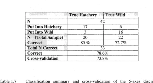
The discriminant function that provided the highest classification level between the two groups was calculated using these five independent variables: (1) Focus; (2) Circuli 1; (3) Circuli 5; (4) Mean circuli width 2-4; and (5) STD 3-6. Of the total usable sample of 42 known origin chinook, the discriminant function classified 36 (85.7%) individuals correctly (Table 1.5A), compared with 21 (50%) expected by chance alone. A Chi’ test between the developed discriminant function and “chance alone” reveals that they are significantly different (i.e. Chi’ is 18.6, P Jess than 0.001). Using a jackknife cross-validation to account for an optimistic apparent error rate (AER) (Minitab 11.21), the discriminant function classified 34 (81%) of the individuals correctly (Table 1.5A).
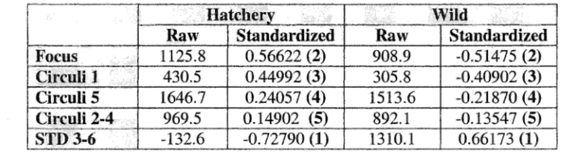
The produced discriminant-identification functions for each group were: (1) Yuatchery=
-63.4 + Focus (1125.8) + Circuli 1 (499.2) + Circuli 5 (1646.7) + STD 3-6 (-132.6) + Mean Circuli Width 2-4 (969.5); and (2) Ywi= - 49.7 + Focus (908.9) + Circuli 1 (305.8) + Circuli
5 (1513.6) + STD 3-6 (1310.1) + Mean Circuli Width 2-4 (892.1). Each set of explanatory variables from an individual are entered into both functions and the function which results in a higher Y value is considered to be the origin of that individual. (See Table 1.5B for specific weights for each variable).To provide the relative predictor level of each of the explanatory variables the data were standardized (i.c. mean of 0, variance of 1). Correlation between the predictors and the discriminant function suggested that the best predictors for distinguishing between hatchery- and wild-produced chinook were: (1) the standard deviation of circuli 3-6; (2) the area of the focus; (3) the width of circuli 1; (4) the width of circuli 5; and (5) the mean width of circuli 2-
4 (Table 1.5B).
To further test the strength of individual variables, discriminant functions were made
by removing one of each of the explanatory variables from the “main” discriminant function
(85.7%). The variable(s) that resulted in the least deviation from the function were circuli 5 and circuli 2-4 (dropped to 83.3% with a cross-validation of 81%) (Table 1.5C) The variable
that resulted in the greatest amount of deviation was STD 3-6 (dropped to 78.6 with a cross validation of 73.8%). Furthermore, discriminant functions were also calculated solely using
each of the explanatory variables to test for the individual discriminating power of each variable. Results from these tests show that at an individual discriminatory level, circuli 1, had the most discriminating power (73.8%) and mean circuli width 2-4 had the least (59.5%) (Table 1.5C).Discriminant function analysis by axes-group
To further test the utility of the 3-axes, which gave a discriminant function of 85.7%
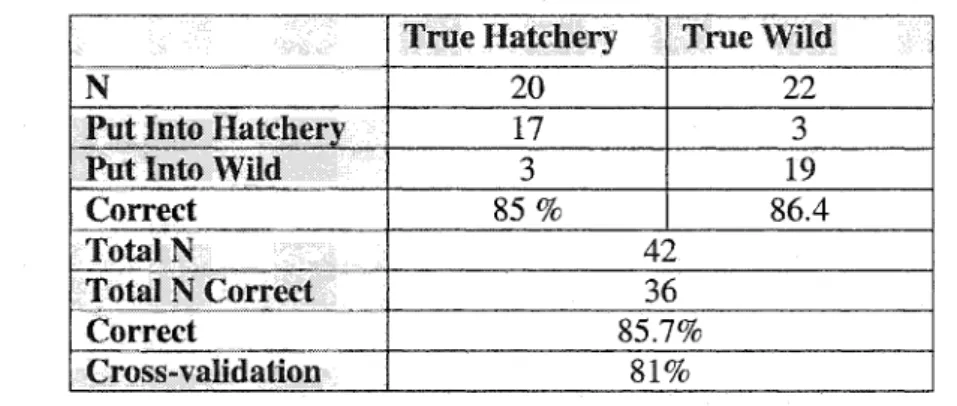
probability and a cross-validation of 81%, discriminant functions were made using measurements from the 1- and 5-axes. The l-axis group gave a discriminant function with
78.6% probability and a cross-validation of 76.2% (Table 1.6), and the 5-axes group had a
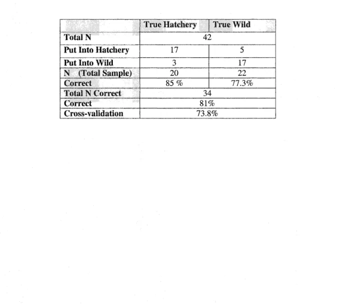
probability level of 81% and a cross-validation of 73.8% (Table 1.7). Thus, the 3-axes group
gave the highest discriminant success.Table 1.5A Classification summary and cross-validation of the discriminant function (N=total number of fish).
Correct T
Table 1.5B Non-standardized (Raw) and standardized relative weights of predictor variables for the linear discriminant function (influence rank highlighted in brackets).
Hatchery Wild
Raw Standardized Raw Standardized
Focus 1125.8 0.56622 (2) 908.9 -0.51475 (2)
Circuli.] 430.5 0.44992 (3) 305.8 -0.40902 (3) Circuli 5 1646.7 0.24057 (4) 1513.6 -0.21870 (4)
| Circuli 2-4 969.5 0.14902 (5) 892.1 -0.13547 (5) STD 3-6 -132.6 -0.72790 (1) 1310.1
0.66173 (1)
Table 1.5C Discriminant functions with one variable removed from the discriminant function (85.7 %) and classification levels for discriminant functions developed with individual variables.
V
ved | validation
Ki 83.3% 78.6%
81.0% 76.2%
83.3% 81.0%
83.3% 81.0%
78.6% 73.8%
Table 1.6 Classification summary and cross-validation of the l-axis discriminant function (N=total number of fish).
Correct
Table 1.7 Classification summary and cross-validation of the 5-axes discriminant function (N=total number of fish).
Put Into Hatchery Put Into
Cross-validation
Discussion Axes comparison
The 3-axes group scale analysis produced the discriminant function with the greatest discriminating power. Specifically, it: (1) provides the best combination of significance levels between variables; (2) has the most reasonable measuring effort when all variables are considered (see below); and (3) produces a discriminant function with the highest discrimination classification. Thus, when attempting to distinguish from scales the origin of Lake Ontario chinook, it is best to use the technique of the 3-axes.
It is estimated that it takes 5 minutes longer to measure 3 axes instead of 1, whereas it
requires an additional 4 minutes to measure 5 axes instead of 3. Thus, the increased levels of
significance gained by measuring along two additional axes (i.e. 1 to 3 axes) is worthwhile,
while there is not a notable gain in significance when measuring two additional axes from 3
to 5 axes. Therefore, overall, we have determined that it is best to use the 3-axes group when analyzing the mean circuli growth of scales.
Growth patterns
The growth of hatchery- and wild-origin chinook salmon, revealed through the pattern on their scales, differed significantly. The results indicate that: (1) hatchery fish were larger
in size than wild fish at the time of platelet formation (i.e. larger focal area). Comparing
focus area, hatchery fish were 16% larger; (2) hatchery fish have greater early growth rates than their wild counterparts (i.e. significantly larger width of individual circuli 1, 5, 6, andsignificantly larger mean widths of circuli 1-6 and 2-4. Overall, comparing the total distance of the first 6 circuli, hatchery fish were 11% larger; and (3) hatchery fish have more consistent early growth patterns (STD 3-6) than wild fish. Comparing STD 3-6, wild fish were 49% more variable than hatchery fish. Since circulus spacing is positively correlated
with growth rate (Bilton 1975), the general appearance of scales from hatchery chinook, with large foci and widely spaced regular circuli, can be directly attributed to increased and more consistent growth rates within the hatchery environment.
Discriminant function
The development of a scale technique to acquire a linear discriminant function that assigns adult chinook salmon on the basis of their natal origin has been successful (85.7 % probability). This study provides the first success at using scale and linear discriminant
function analysis to distinguish between hatchery and wild chinook salmon in the Great
Lakes. Different developmental, and possibly genetic forces, experienced in the early growth period of the lives of the two groups resulted in scale characteristics that would allow classification of their origin. Such analysis can be performed at any age, as long as the scales are large enough to be analyzed (i.e. after a few months of growth). Using discriminant function analysis based solely on early scale characteristics, we were able to assess the origin of adult chinook salmon collected in the Credit River during the fall spawning run of 2001 (Chapter 2). The discriminant function had a classification probability of 85.7 % with a jackknife cross-validation, indicating that 81 % of the known-origin juveniles were correctly classified as to origin.It is important to address the fact that there were some limitations in the data used in
the development of the discriminant function. Specifically: (1) Ringwood Hatchery juveniles and Wilmot Creek adults were both sampled in single years, therefore the growth patterns observed do not represent the mean pattern across several years. This is a potential issue since the scale growth pattern is influenced by environmental factors in the wild and the possibility exists that scales sampled in another year characterized by different environmental factors (the hatchery should remain consistent on an annual basis) may show additionalsignificantly different variables. Thus, it would be beneficial to use the mean of growth
patterns from different years when using scales as representative for each group; (2) Wilmot Creek adults were assumed to be the product of natural reproduction. Although it has never
been scientifically proven, it is believed by OMNR that the majority (~99%) of returning adults to Wilmot Creek are those that were produced in the wild. There is always the possibility of hatchery strays entering the river, although this is not believed to be significantsince stocking does not occur in close proximity to that river. Finally, (3) adults collected
from Wilmot Creek may be a biased sample since they may not be representative of the average early growth of juveniles from wild production. Specifically, the returning adults may correspond to those that had the best growth during the juvenile stage and are the individuals that most likely survived and able to spawn. [f this is true, when compared to the juvenile growth patterns of hatchery fish, the representative mean growth patterns of wild juveniles would likely have yet smaller foci area and even more reduced circuli width.Implications
The analysis of scale variables revealed that scale analysis can be used as a tool for identifying origin of chinook in Lake Ontario. In general, scale analysis has several advantages over other discriminatory techniques, for example, physical tags. This is especially true when dealing with large populations that span wide geographic areas. For example, the magnitude of many fish-stocking programs makes the use of coded wire tags impractical and unfeasible. This is because hatchery releases are often too numerous (several hundred thousand to several million) to apply tags or other physical labels, such as fin clips or thermal marks, without incurring high financial cost and/or mortality levels. Each year OMNR releases approximately half a million chinook into the Lake Ontario watershed.
Another significant disadvantage of physical tags is that they require placement on the animal
prior to its capture, and hence the animal must be handled. This is in direct contrast to scale analysis, which allow researchers to study an individual at any time after capture. Genetic markers have also shown promise for stock identification in some fisheries applications (e.g.
Letcher and King 1999). Yet, the accuracy of identifying individual fish to specific stocks based upon DNA variation is limited when many stocks are considered and few loci are available (Beacham et al. 1996). Additionally, the genetic structure of some populations such as salmon can exhibit significant temporal variability (Garant et al. 2000) and can be significantly altered as a result of interactions between hatchery and wild stocks (Kennedy et al, 2000). The use of stable isotopes has also become popular recently, however they have some disadvantages. First, there is often a high probability of contamination of the sample during processing (Hobson and Wassenaar 1999); second, there is the problem of pollution and any changes that may arise among the geology in certain areas; third, the isotopic composition of salmon from other areas could be complicated by the mixing of waters from different tributaries and the local control of strontium isotopic values by bedrock in each
drainage (Harrington et al. 1998); and last, the process is often very expensive when
compared to scale analysis. Although there are a variety of advantages with using scale analysis, there are a few shortcomings with this process. These include: (1) the length of time required to complete the analysis. For example, physical tags require significantly less analysis; and (2) the interpretation component that arises when an individual measures, whichmay influence the data. For example, the center of the focus as well as the end of each
circulus is determined by the individual.On the whole, scale analysis can be utilized as a very powerful tool for discriminating the origin of mixed samples. Specifically, the results of this study indicate that the
measurement of scale patterns along an additional two axes provides a higher resolving
power than the traditional method of single axis scale analysis. Thus, it is possible thatprevious unsuccessful studies attempting to distinguish hatchery and wild fish through scale analysis in the Great Lakes may have been hindered by the use of only one axis. An example of such a study is that of Carl (1982) who aimed to distinguish known Lake Michigan wild and hatchery chinook juveniles through the use of scale parameters but was unable to develop a discriminant function that confidently separated the two groups (66%). The study from Carl (1982) also suggests a problem in the choice of the variables measured and utilized for his discriminant analysis (i.e. # of pre-lake circuli, focus area, and pre-lake circulus spacing).
In particular, he did not use the variable (STD 3-6) that had a notable influence on the discriminant function developed in this study.
These results provide a foundation for the determination of unknown origin
individuals in samples of chinook collected in Lake Ontario. Future chinook salmon studies in Lake Ontario that would benefit from these results include: (1) investigation of the proportions of hatchery and wild chinook in Lake Ontario, which would provide fisheries managers with a better understanding of the chinook population; (2) investigation of the proportion of hatchery and wild chinook in specific tributaries of Lake Ontario (e.g. Credit River), which would allow for a better understanding of the production of each river; and (3) studies of phenotypic and genotypic traits of wild and hatchery fish, which would allow forthe understanding of the very recent evolutionary history of these fish in Lake Ontario.
Summary
The development of a scale technique to acquire a linear discriminant function that