FINITE ELEMENT APPROXIMATION OF THE VIBRATION
PROBLEM FOR A TIMOSHENKO CURVED ROD
E. HERN ´ANDEZ∗, E. OT ´AROLA†, R. RODR´IGUEZ‡, AND F. SANHUEZA§
Abstract. The aim of this paper is to analyze a mixed finite element method for computing the vibration modes of a Timoshenko curved rod with arbitrary geometry. Optimal order error estimates are proved for displacements and rotations of the vibration modes, as well as a double order of convergence for the vibration frequencies. These estimates are essentially independent of the thickness of the rod, which leads to the conclusion that the method is locking free. A numerical test is reported in order to assess the performance of the method.
1. Introduction
It is very well known that standard finite elements applied to models of thin structures, like beams, rods, plates and shells, are subject to the so-called lock-ing phenomenon. This means that they produce very unsatisfactory results when the thickness of the structure is small with respect to the other dimensions of the structure (see for instance [4]). From the point of view of the numerical analysis, this phenomenon usually reveals itself in that the a priori error estimates for these methods depend on the thickness of the structure in such a way that they degener-ate when this parameter becomes small. To avoid locking, special methods based on reduced integration or mixed formulations have been devised and are typically used to date (see, for instance, [5]).
Very likely, the first mathematical piece of work dealing with numerical locking and how to avoid it is the paper by Arnold [1], where a thorough analysis for the Timoshenko beam bending model is developed. In that paper, it is proved that locking arises because of the shear terms and a locking-free method based on a mixed formulation is introduced and analyzed. It is also shown that this mixed method is equivalent to use a reduced-order scheme for the integration of the shear terms in the primal formulation.
Subsequently, several methods to avoid locking on different models of circular arches were developed by Kikuchi [12], Loula et al. [14] and Reddy and Volpi
2000 Mathematics Subject Classification. 65N25, 65N30, 74K10.
Key words. Timoshenko curved rods, finite element method, vibration problem.
∗Partially supported by FONDECYT grant 1070276 and USM grant 12.05.26.
†Partially supported by USM grant 12.05.26.
‡Partially supported by FONDAP in Applied Mathematics.
[15]. The analysis of the latter was extended by Arunakirinathar and Reddy in [2] to Timoshenko rods of rather arbitrary geometry. An alternative approach to deal with this same kind of rods was developed and analyzed by Chapelle in [6], where a numerical method based on standard beam finite elements was used to approximate the rod.
All the above references deal only with load problems. The literature devoted to the dynamic analysis of rods is less rich. There exist a few papers introducing finite element methods and assessing their performance by means of numerical experiments (see [10,13] and references therein). Papers dealing with the numerical analysis of the eigenvalue problems arising from the computation of the vibration modes for thin structures are much less frequent (among them we mention [7,
8], where MITC methods for computing bending vibration modes of plates were analyzed). One reason for this is that the extension of mathematical results from load to vibration problems is not quite straightforward for mixed methods.
In this paper we adapt to the vibration problem the mixed finite element method proposed and analyzed by Arunakirinathar and Reddy in [2] for the load problem for elastic curved rods. With this purpose, we settle the corresponding spectral problem by including the mass terms arising from displacement and rotational inertia in the model, as proposed in [10]. Our assumptions on the rods are slightly weaker than those in [2]. On the one hand we allow for non-constant geometric and physical coefficients varying smoothly along the rod. On the other hand, we do not assume that the Frenet basis associated with the line of cross-section centroids is a set of principal axes. We prove that the resulting method yield optimal order approximation of displacements and rotations of the vibration modes, as well as a double order of convergence for the vibration frequencies. Under mild assumptions, we also prove that the error estimates do not degenerate as the thickness becomes small, which allow us to conclude that the method is locking free.
The outline of the paper is as follows. In Sect.2, we introduce the basic geometric and physical assumptions to settle the vibration problem for a Timoshenko rod of arbitrary geometry. The resulting spectral problem is shown to be well posed. Its eigenvalues and eigenfunctions are proved to converge to the corresponding ones of the limit problem as the thickness of the rod goes to zero, which corresponds to a Bernoulli-like rod model. The finite element discretization with piecewise polynomials of arbitrary degree is introduced and analyzed in Sect. 3. Optimal orders of convergence are settled for the eigenfunctions, as well as a double order for the eigenvalues and, whence, for the vibration frequencies. All these error estimates are proved to be independent of the thickness of the rod, which allow us to conclude that the method is locking-free. In Sect.4, we report a numerical test, which allows assessing the performance of the lowest-degree method.
2. The vibration problem for an elastic rod of arbitrary geometry
the line of centroids. The curve is parametrized by its arc lengths∈I:= [0, L],L
being the total length of the curve.
We recall some basic concepts and definitions; for further details see [2], for instance. We use standard notation for Sobolev spaces and norms.
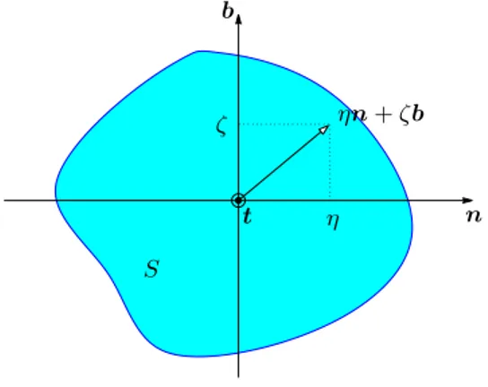
The basis in which the equations are formulated is the Frenet basis consisting oft,nandb, which are the tangential, normal and binormal vectors of the curve, respectively. These vectors change smoothly from point to point and form an orthogonal basis ofR3at each point.
LetS denote a cross-section of the rod. We denote by (η, ζ) the coordinates in the coordinate system{n,b}of the plane containing S (see Fig.2.1).
η ζ ηn+ζb
t b
n
S
Fig. 2.1. Cross-section. Coordinate system.
The geometric properties of the cross-section are determined by the following parameters (recall that the first moments of area,RSη dη dζ andRSζ dη dζ, vanish, because the center of coordinates is the centroid ofS):
• the area of S: A:=RS dη dζ;
• the second moments of area with respect to the axisR n and b: In := Sζ
2dη dζ andIb:=R
Sη
2dη dζ, respectively;
• the polar moment of area: J :=RS η2+ζ2dη dζ =In+Ib; • Inb:=RSηζ dη dζ.
These parameters are not necessarily constant, but they are assumed to vary smoothly along the rod. For a non-degenerate rod,Ais bounded above and below far from zero. Consequently, the same happens for the area moments,In,Ib and
J.
axes, so thatInb does not necessarily vanish. In any case, it is straightforward to
prove that the matrix
In −Inb −Inb Ib
is always positive definite.
Vector fields defined on the line of centroids will be always written in the Frenet basis:
v=v1t+v2n+v3b, with v1, v2, v3: I−→R.
We emphasize thatv1,v2andv3are not the components ofvin a fixed basis ofR3, but in the Frenet basis{t,n,b}, which changes from point to point of the curve.
Since t, nand b are smooth functions of the arc-length parameters, we have that
v′=v1′t+v′2n+v3′b+v1t′+v2n′+v3b′.
If we denote
˙
v:=v1′t+v2′n+v3′b, (2.1)
then, by using theFrenet-Serret formulas (see, for instance, [2]), there holds
v′= ˙v+ Γtv, with Γ(s) :=
0 κ(s) 0
−κ(s) 0 τ(s) 0 −τ(s) 0
,
where κ and τ are the curvature and the torsion of the rod, which are smooth functions of s, too. Therefore, v = v1t+v2n+v3b ∈ H1(I)3 if and only if
vi∈L2(I) and ˙vi∈L2(I),i= 1,2,3.
Since we will confine our attention to elastic rods clamped at both ends, we proceed as in [2] and consider
V:=v∈L2(I)3: ˙v∈L2(I)3andv(0) =v(L) =0 , endowed with its natural norm
kvk1:= "Z L
0
|v|2+|v˙|2ds
#1/2
;
namely, V is the space of vector fields defined on the line of centroids such that their components in the Frenet basis are in H1
0(I).
We will systematically use in what follows the total derivativev′ = ˙v+Γtv. Since
t, nand bare assumed to be smooth functions, kv′k0 is a norm onV equivalent to k·k1(see [2, Theorem 3.1]). This is the reason why we denotek·k1 the norm of
V. However, the total derivative v′ should be distinguished from the vector ˙v of derivatives of the components ofv in the Frenet basis, as defined by (2.1).
positive coefficients. These coefficients are not necessarily constant; they are al-lowed to vary along the rod, but they are also assumed to be smooth functions of the arc-lengths.
We consider the problem of computing the free vibration modes of an elastic rod clamped at both ends. The variational formulation of this problem consists in finding non-trivial (u,θ)∈W:=V×V andω >0 such that
Z L
0
Eθ′·ψ′ds+ Z L
0
D(u′−θ×t)·(v′−ψ×t)ds
=ω2
Z L
0
ρAu·vds+ Z L
0
ρJθ·ψds !
∀(v,ψ)∈W, (2.2)
whereωis the vibration frequency anduandθ are the amplitudes of the displace-ments and the rotations, respectively (see [10]). The coefficients D, E and J are 3×3 matrices, which in the Frenet basis are written as follows:
D:=
EA 0 0
0 k1GA 0
0 0 k2GA
,
E:=
GJ 0 0
0 EIn −EInb
0 −EInb EIb
and J:=
J 0 0
0 In −Inb
0 −Inb Ib
.
In [10], as in most references ([2, 6]), the Frenet basis is assumed to be a set of principal axes, so thatInb= 0 and the three matrices above are diagonal. We do not make this assumption in this paper.
Remark2.2. The vibration problem above can be formally obtained from the three-dimensional linear elasticity equations as follows: According to the Timoshenko hypotheses, the admissible displacements at each pointηn+ζb∈S (see Fig.2.1) are of the form u+θ ×(ηn+ζb), with u, θ, n and b being functions of the arc-length coordinates. Test and trial displacements of this form are taken in the variational formulation of the linear elasticity equations for the vibration problem of the three-dimensional rod. By integrating over the cross-sections and multiplying the shear terms by correcting factorsk1 andk2, one arrives at problem (2.2).
With this purpose, we introduce the following non-dimensional parameter, char-acteristic of the thickness of the rod:
d2:= 1
L
Z L
0 J AL2ds.
By defining
λ:=ω
2ρ
d2 , Db :=
1
d2D, Eb:=
1
d4E, bJ:=
1
d4J and Ab:= A d2,
Problem (2.2) can be equivalently written as follows:
ProblemP: Find non-trivial(u,θ)∈W andλ∈Rsuch that Z L
0
b
Eθ′·ψ′ds+ 1
d2
Z L
0
b
D(u′−θ×t)·(v′−ψ×t)ds
=λ
Z L
0
b
Au·vds+d2
Z L
0
bJθ·ψds
!
∀(v,ψ)∈W.
The values of interest of d are obviously bounded above, so we restrict our attention to d∈(0, dmax]. The coefficients of the matricesDb, bEandbJ, as well as
b
A, are assumed to be functions of s which do not vary withd. This corresponds to considering a family of problems where the size of the cross-sections at all point of the line of centroids are uniformly scaled byd, while their shapes as well as the geometry of the curve and the material properties remain fixed.
Remark 2.3. Matrices Db, bEandbJ are positive definite for alls∈I, the last two because of Remark2.1. Moreover, since all the coefficients are continuous functions ofs, the eigenvalues of each of these matrices are uniformly bounded below away from zero for alls∈I.
Remark 2.4. The eigenvalues λ of Problem P are strictly positive, because of the symmetry and the positiveness of the bilinear forms on its left and right-hand sides. The positiveness of the latter is a straightforward consequence of Remark2.3, whereas that of the former follows from the ellipticity of this bilinear form inW. This can be proved by using Remark2.3again and proceeding as in the proof of [2, Lemma 3.4 (a)], where the same result appears for particular constant coefficients (see also [6, Proposition 1]).
We introduce the scaled shear stressγ:= 1
d2Db(u
′−θ×t) to rewrite ProblemP
as follows:
b
Eθ′,ψ′+ (γ,v′−ψ×t) =λhAbu,v+d2bJθ,ψi ∀(v,ψ)∈W,
γ= 1
d2Db(u
′
−θ×t),
where (·,·) denotes the L2(I)3 inner product.
To analyze the approximation of this problem, we introduce the operator
defined byT(f,φ) := (u,θ), where (u,θ)∈W is the solution of the associated load problem:
b
Eθ′,ψ′+ (γ,v′−ψ×t) =Abf,v+d2bJφ,ψ ∀(v,ψ)∈W, (2.3) γ= 1
d2Db(u
′
−θ×t). (2.4)
The existence and uniqueness of the solution of this problem was analyzed in [2, Theorem 3.3] in case of particular constant coefficients and in [6, Proposition 2] for another equivalent formulation. Taking into account that (2.4) can be equivalently written as follows:
(u′−θ×t,q)−d2Db−1γ,q= 0 ∀q∈Q:= L2(I)3,
we note that the load problem falls in the framework of the mixed formulations considered in [5]. In this reference, the results from [1] are extended to cover this kind of problems. In particular, according to [5, Theorem II.1.2], to prove the well posedness it is enough to verify the classical properties of mixed problems:
i) ellipticity in the kernel: ∃α >0 such that
b
Eψ′,ψ′≥αkvk2
1+kψk 2 1
∀(v,ψ)∈W0,
where W0:={(v,ψ)∈W : v′−ψ×t= 0 inI};
ii) inf-sup condition: ∃β >0 such that
sup
(0,0)6=(v,ψ)∈W
(q,v′−ψ×t)
kvk1+kψk1 ≥βkqk0 ∀q∈Q.
Property (i) has been proved in [2, Lemma 3.6] forEbbeing the identity matrix. The extension toEbpositive definite uniformly insis quite straightforward. Property (ii) has been proved in [2, Lemma 3.7]. An alternative simpler proof of an equivalent inf-sup condition appears in [6, Proposition 2].
Therefore, according to [5, Theorem II.1.2], problem (2.3)–(2.4) has a unique solution (u,θ,γ)∈W×Qand this solution satisfies
kuk1+kθk1+kγk0≤C kfk0+d2kφk0.
Here and thereafter,Cdenotes a strictly positive constant, not necessarily the same at each occurrence, but always independent ofdand of the mesh-sizeh, which will be introduced in the next section.
Because of the estimate above and the compact embedding H1(I) ֒→ L2(I),
the operator T is compact. Moreover, by substituting (2.4) into (2.3), from the symmetry of the resulting bilinear forms, it is immediate to show thatT is self-adjoint with respect to the ‘weighted’ L2(I)3×L2(I)3 inner product in the
Note thatλis a non-zero eigenvalue of ProblemPif and only ifµ:= 1/λis a non-zero eigenvalue ofT, with the same multiplicity and corresponding eigenfunctions. Recall that these eigenvalues are strictly positive (cf. Remark2.4).
Next, we defineT0by means of the limit problem of (2.3)–(2.4) asd→0:
T0: L2(I)3×L2(I)3−→L2(I)3×L2(I)3,
whereT0(f,φ) := (u0,θ0)∈W is such that there existsγ0∈Qsatisfying:
b
Eθ′0,ψ′+ (γ0,v′−ψ×t) =Abf,v ∀(v,ψ)∈W,
u′0−θ0×t=0.
The above mentioned existence and uniqueness results from [2, Theorem 3.3] and [6, Proposition 2] covers this problem as well, in case of constant coefficients. As stated above, the proofs can be readily extended to our case.
It is proved in [9] thatTt converge in norm to T0. The next theorem follows from this fact and classical results from spectral perturbation theory (see [11]):
Lemma 2.1. Letµ0>0be an eigenvalue ofT0of multiplicitym. LetDbe any disc
in the complex plane centered atµ0and containing no other element of the spectrum of T0. Then, for dsmall enough,D contains exactlym eigenvalues of T (repeated according to their respective multiplicities). Consequently, each eigenvalue µ0>0
of T0 is a limit of eigenvalues µof T, asd goes to zero.
Moreover, for any compact subset K of the complex plane not intersecting the spectrum ofT0, there existsdK >0 such that for all d < dK,K does not intersect
the spectrum ofT, either.
3. Finite elements discretization
Two different finite element discretizations of the load problem for Timoshenko curved rods have been analyzed in [2] and [6]. The two methods differ in the variables being discretized: the components of vector fieldsv in the Frenet basis,
v1,v2 andv3, are discretized by piecewise polynomial continuous functions in [2]; instead, in [6], the discretized variable is the vector fieldv=v1t+v2n+v3b. We follow the approach in [2].
Consider a family{Th}of partitions of the intervalI,Th: 0 =s0< s1<· · ·<
sn=L, with mesh-sizeh:= maxj=1,...,n(sj−sj−1). We define the following finite
element subspaces ofV andQ, respectively:
Vh:=
v∈V: vi|[sj−1,sj]∈ Pr, j= 1, . . . , n, i= 1,2,3 ,
Qh:=q∈Q: qi|[sj−1,sj] ∈ Pr−1, j= 1, . . . , n, i= 1,2,3 ,
wherevi,i= 1,2,3, are the components ofvin the Frenet basis,Pkare the spaces of polynomials of degree lower or equal tok, andr≥1.
ProblemPh: Find non-trivial(uh,θh,γh)∈Wh×Qh andλh∈Rsuch that:
b
Eθ′h,ψ′h+ (γh,v′h−ψh×t) =λh h
b
Auh,vh+d2bJθh,ψhi
∀(vh,ψh)∈Wh, (u′h−θh×t,qh)−d2Db−1γh,qh= 0 ∀qh∈Qh.
In the same manner as in the continuous case, we introduce the operator
Th: L2(I)3×L2(I)3−→L2(I)3×L2(I)3,
defined byTh(f,φ) := (uh,θh), where (uh,θh,γh)∈Wh×Qh is the solution of the associated discrete load problem:
b
Eθ′h,ψ′h+ (γh,v′h−θh×t) =Abf,vh+d2bJφ,ψh
∀(vh,ψh)∈Wh, (3.1) (u′h−θh×t,qh)−d2
b
D−1γh,qh
= 0 ∀qh∈Qh. (3.2)
Problem (3.1)–(3.2) falls in the framework of the discrete mixed formulations considered in [5, Section II.2.4]. In order to apply Proposition II.2.11 from this reference to conclude well-posedness of this discrete problem and error estimates, it is enough to verify the following classical properties, forhsmall enough:
i) ellipticity in the discrete kernel: ∃α∗>0, independent ofh, such that
b
Eψ′h,ψ′h≥α∗kvhk2
1+kψhk
2 1
∀(vh,ψh)∈W0h,
where W0h:={(vh,ψh)∈Wh: (qh,v′h−ψh×t) = 0 ∀qh∈Qh}; ii) discrete inf-sup condition: ∃β∗>0, independent ofh, such that
sup
(0,0)6=(vh,ψh)∈Wh
(qh,v′h−ψh×t)
kvhk1+kψhk1 ≥
β∗kqhk0 ∀qh∈Qh.
Property (i) has been proved in [2, Lemma 4.2] forEbbeing the identity matrix and
h >0 sufficiently small. The extension tobEpositive definite uniformly insis quite straightforward. Property (ii) has been proved in [2, Lemma 4.3]. An alternative simpler proof of this condition can be found in [9, Lemma 6.2].
On the other hand, (3.4) is obtained by adapting to our case the duality argu-ment used to prove [6, Theorem 2]. Therefore, the following theorem follows:
Theorem 3.1. For sufficiently small h > 0, problem (3.1)–(3.2) has a unique
solution(uh,θh,γh)∈Wh×Qh. This solution satisfies
kuhk1+kθhk1+kγhk0≤C kfk0+d2kφk0
,
Let (u,θ,γ) ∈ W ×Q be the solution of (2.3)–(2.4). If f,φ ∈ Hk−1(I)3 ,
1≤k≤r, then
ku−uhk1+kθ−θhk1+kγ−γhk0 ≤ Chk kfkk−1+d2kφkk−1
, (3.3)
ku−uhk0+kθ−θhk0 ≤ Chk+1 kfkk−1+d2kφkk−1, (3.4)
with C >0 independent ofhandd.
By adding (3.1) and (3.2), from the symmetry of the resulting bilinear forms, it is immediate to show thatThis self-adjoint with respect to the ‘weighted’ L2(I)3× L2(I)3 inner product in the right-hand side of (3.1). Therefore, apart ofµ
h = 0, the spectrum ofThconsists of a finite number of finite-multiplicity real eigenvalues with ascent 1.
Once more the spectrum of the operator Th is related with the eigenvalues of the spectral problem Ph: λh is a non-zero eigenvalue of this problem if and only if µh := 1/λh is a non-zero eigenvalue of Th, with the same multiplicity and corresponding eigenfunctions. It is simple to prove that these eigenvalues are strictly positive. Moreover, the eigenvalues cannot vanish. In fact, according to the expression above, since Eb and Db are positive definite (see Remark 2.3),
λh = 0 implies γh = 0. Then, the second equation of Problem Ph implies that
(uh,θh)∈W0h and, hence,uhandθh vanish because of property (i).
Our aim is to use the spectral theory for compact operators (see [3], for instance) to prove convergence of the eigenvalues and eigenfunctions ofTh towards those of
T. However, some further considerations will be needed to show that the error estimates do not deteriorate asd becomes small. With this purpose, we will use the following result:
k(T−Th)(f,φ)k1≤Ch kfk0+d2kφk0
,
which follows from (3.3) withk= 1. As a consequence of this estimate,Thconverges in norm toT ashgoes to zero. Hence, standard results of spectral approximation (see for instance [11]) show that ifµis an eigenvalue ofT with multiplicitym, then exactlym eigenvaluesµ(1)h , . . . , µ(hm) ofTh (repeated according to their respective multiplicities) converge to µ.
The estimate above can be improved when the source term is an eigenfunction (u,θ) ofT. Indeed, in such a case, for all k≥2 anddsufficiently small,
kukk+kθkk+kγkk−1≤C kuk0+d 2
kθk0,
with C depending onk and on the eigenvalue of T associated with (u,θ). Note that in principle the constantC should depend also on d, because the eigenvalue does it. However, according to Lemma2.1, for dsufficiently small we can choose
C independent ofd. Hence, from (3.3)–(3.4) with k=r, we obtain:
k(T−Th) (u,θ)k1 ≤ Chrk(u,θ)k1, (3.5)
We remind the definition of the gap or symmetric distance δbk between closed subspacesY andZ ofW in normk·kk,k= 0,1:
b
δk(Y,Z) := max{δk(Y,Z), δk(Z,Y)}, with
δk(Y,Z) := sup
(v,ψ)∈Y
k(v,ψ)kk=1
" inf
(vb,ψ)b ∈Z
(v−bv,ψ−ψb) k
#
.
For the sake of simplicity we state our results for eigenvalues ofT converging to a simple eigenvalue ofT0 as d→ 0. The following theorem yields d-independent error estimates for the approximate eigenvalues and eigenfunctions. Its proof is a consequence of (3.5)–(3.6), [3, Theorem 7.1 and 7.2] and Lemma2.1.
Theorem 3.2. Let µ be an eigenvalue of T converging to a simple eigenvalue µ0
of T0 as d tends to zero, Letµh be the eigenvalue of Th that converges to µ as h
tends to zero. LetE and Eh be the corresponding eigenspaces. Then, for dand h
small enough,
b
δ1(E,Eh) ≤ Chr, b
δ0(E,Eh) ≤ Chr+1,
withC >0independent of dandh.
This theorem yields optimal order error estimates for the approximate eigenfunc-tions in normsk·k1 andk·k0. An optimal double order holds for the approximate eigenvalues. In fact, the following theorem has been proved in [9, Theorem 3.4] by adapting to our problem a standard argument for variationally posed eigenvalue problems (see [3, Lemma 9.1], for instance).
Theorem 3.3. Let λ= 1
µ andλh=
1
µh, withµandµh as in Theorem3.2. Then,
ford andh small enough,
|λ−λh| ≤Ch2r,
withC >0independent of dandh.
4. Numerical results
We report in this section the results of a numerical test computed with amatlab code implementing the finite element method described above. We have used the lowest possible order: r = 1; namely, piecewise linear continuous elements for the displacementsuh and the rotations θh, and piecewise constant discontinuous elements for the shear stressesγh.
We have computed the vibration modes with lowest frequencies ωh:=√λ h for a helical rod. We have considered a helix with five turns, clamped at both ends. The equation of the helix centroids line parametrized by its arc-length is as follows:
r(s) =Acos s
n, Asin s n, C
s n
, with n=pA2+C2; (4.1)
the curvature isκ=A/n2, the torsionτ=C/n2, and the length of the eight-turns
side-lengthb= 20 cm as the cross section of the rod. Thus, the thickness parameter is in this cased= 0.0026. Figure4.1 shows the undeformed helix.
Fig. 4.1. Undeformed helical rod.
We have computed the lowest vibration frequencies ωh
1 < ω2h < ω3h < · · · by
using uniform meshes ofN elements, with different values ofN. We have used the following physical parameters, which correspond to steel:
• elastic moduli: E= 2.1×10⁶kgf/cm2(1 kgf = 980 kg cm/s2); • Poisson coefficient: ν = 0.3;
• density: ρ= 7.85×10⁻³kg/cm3; • correction factors: k1=k2= 1.
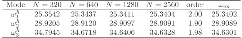
Since no analytical solution is available for this rod, we have estimated the order of convergence by means of a least squares fitting. Table 4.1 shows the lowest vibration frequencies computed on successively refined meshes. It also includes the computed orders of convergence and extrapolated ‘exact’ vibration frequenciesωex.
Table 4.1. Angular vibration frequencies of a helical rod.
Mode N = 320 N = 640 N = 1280 N= 2560 order ωex
ωh1 25.3542 25.3437 25.3411 25.3404 2.00 25.3402 ωh2 28.9205 28.9120 28.9097 28.9091 1.90 28.9089 ωh3 34.7945 34.6718 34.6406 34.6328 1.98 34.6301
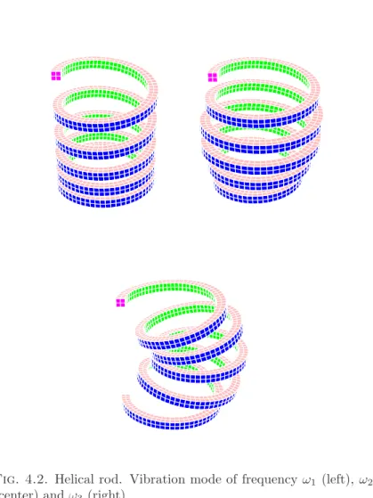
Figure4.2show the lowest-frequency vibration modes. The first one is a typical spring mode, the second one is an extensional mode, and the third one is a kind of ‘phone rope’ vibration mode.
Fig. 4.2. Helical rod. Vibration mode of frequencyω1 (left),ω2
(center) and ω3(right).
References
[1] Arnold, D.N.,Discretization by finite elements of a model parameter dependent problem. Numer. Math., 37 (1981) 405–421.1,2,2
[2] Arunakirinathar, K., Reddy, B.D.,Mixed finite element methods for elastic rods of arbi-trary geometry, Numer. Math., 64 (1993) 13–43.1,2,2,2,2.4,2,3,3
[3] Babuˇska. I., Osborn, J.,Eigenvalue problems, in: Handbook of Numerical Analysis, Vol II. Ciarlet, P.G., Lions, J.L. (eds.), North Holland, Amsterdam, 1991, pp. 641–687.3,3,3
[5] Brezzi, F., Fortin, M.,Mixed and Hybrid Finite Element Methods, Springer-Verlag, New York, 1991.1,2,3
[6] Chapelle, D.,A locking-free approximation of curved rods by straight beam elements, Nu-mer. Math., 77 (1997) 299–322.1,2,2.4,2,3,3
[7] Dur´an, R., Hervella-Nieto, L., Liberman, E., Rodr´ıguez, R., Solomin, J., Approxi-mation of the vibration modes of a plate by Reissner-Mindlin equations, Math. Comp., 68 (1999) 1447–1463.1
[8] Dur´an, R., Hern´andez, E., Hervella-Nieto, L., Liberman, E., Rodr´ıguez, R.,Error es-timates for low-order isoparametric quadrilateral finite elements for plates, SIAM J. Numer. Anal., 41 (2003) 1751–1772.1
[9] Hern´andez, E., Ot´arola, E., Rodr´ıguez, R., Sanhueza, F.,Approximation of the vibra-tion modes of a Timoshenko curved rod of arbitrary geometry, IMA J. Numer. Anal. (to appear).2,3,3
[10] Karami, G., Farshad, M., Yazdchi, M.,Free vibrations of spatial rods - a finite-element analysis. Comm. Appl. Numer. Methods, 6 (1990) 417–428.1,2
[11] Kato, T.,Perturbation Theory for Linear Operators, Springer Verlag, Berlin, 1995.2,3
[12] Kikuchi, F.,Accuracy of some finite element models for arch problems, Comput. Methods Appl. Mech. Engrg., 35 (1982) 315–345.1
[13] Litewka, P., Rakowski, J., Free vibrations of shear-flexible and compressible arches by FEM., Internat. J. Numer. Methods Eng., 52 (2001) 273–286.1
[14] Loula, A.F.D., Franca, L.P., Hughes, T.J.R., Miranda, I,Stability, convergence and accuracy of a new finite element method for the circular arch problem, Comput. Methods Appl. Mech. Engrg., 63 (1987) 281-303.1
[15] Reddy, B.D., Volpi, M.B., Mixed finite element methods for the circular arch problem, Comput. Methods Appl. Mech. Engrg., 97 (1992) 125–145.1
E. Hern´andez
Departamento de Matem´atica,
Universidad T´ecnica Federico Santa Mar´ıa, Casilla 110-V, Valpara´ıso, Chile.
E. Ot´arola
Departamento de Matem´atica,
Universidad T´ecnica Federico Santa Mar´ıa, Casilla 110-V, Valpara´ıso, Chile.
R. Rodr´ıguez
Departamento de Ingenier´ıa Matem´atica, Universidad de Concepci´on,
Casilla 160-C, Concepci´on, Chile. [email protected]
F. Sanhueza
Departamento de Ingenier´ıa Matem´atica, Universidad de Concepci´on,
Casilla 160-C, Concepci´on, Chile. [email protected]