UNIVERSIDAD DE CONCEPCI ´ ON
Centro de Investigaci´ on en Ingenier´ıa Matem´ atica (CI 2 MA)
A posteriori virtual element method for the acoustic vibration problem
Felipe Lepe, David Mora, Gonzalo Rivera, Iv´ an Vel´ asquez
PREPRINT 2022-17
SERIE DE PRE-PUBLICACIONES
VIBRATION PROBLEM
F. LEPE, D. MORA, G. RIVERA, AND I. VEL ´ASQUEZ
Abstract. In two dimensions, we propose and analyze an a posteriori error estimator for the acoustic spectral problem based on the virtual element method in H(div; Ω). Introducing an auxiliary unknown, we use the fact that the primal formulation of the acoustic problem is equivalent to a mixed formulation, in order to prove a superconvergence result, necessary to despise high order terms. Under the virtual element approach, we prove that our local indicator is reliable and globally efficient in the L2-norm. We provide numerical results to assess the performance of the proposed error estimator.
1. Introduction
One of the most important subjects in the development of numerical methods for partial differential equations is the a posteriori error analysis, since it allows dealing with singular solutions that arise due, for instance, geometrical features of the domain or some particular boundary conditions, among others. In this sense, and in particular for eigenvalue problems arising from problems related to solid and fluid mechanics and electromagnetism, just to mention some possible applications, the a posteriori analysis has taken relevance in recent years. (see [2, 12, 14, 11, 21, 22, 33, 35, 38, 39] and the references therein).
The virtual element method (VEM), introduced in [4], has shown remarkable results in different problems, and particularly for solving eigenproblems, showing great accuracy and flexibility in the approximation of eigenvalues and eigenfunctions. We mention [18, 19, 24, 25, 26, 27, 28, 31, 30, 32, 33, 34, 36] as recent works on this topic.
The acoustic vibration problem appears in important applications in engineering. In fact, it can be used to design of structures and devices for noise reduction in aircraft or cars mainly related with solid-structure interaction problems, among others important applications. In the last years, several numerical methods have been developed in order to approximate the eigenpairs of the associated spec- tral problem. In particular, a virtual element discretization has been proposed in [9]. It is well known that one of the most important features of the virtual element method is the efficient computational implementation and the flexibility on the geometries for meshes, where precisely adaptivity strategies can be implemented in an easy way. In fact, the hanging nodes that appear in the refinement of some element of the mesh, can be treated as new nodes since adjacent non matching element interfaces are acceptable in the VEM. Recent research papers report interesting advantages of the VEM in the a posteriori error analysis and adaptivity for source problems. We refer to [7, 16, 17, 37] and the references therein, for instance, for a further discussion. On the other hand, a posteriori error analysis
2000Mathematics Subject Classification. 65N30, 65N25, 70J30, 76M25.
Key words and phrases. virtual element method, acoustic vibration problem, polygonal meshes, a posteriori error estimates, superconvergence.
The first author has been partially supported by DICREA through project 2120173 GI/C Universidad del B´ıo-B´ıo and ANID-Chile through FONDECYT project 11200529, Chile.
The second author was partially supported by DICREA through project 2120173 GI/C Universidad del B´ıo-B´ıo, by the National Agency for Research and Development, ANID-Chile through FONDECYT project 1220881, by project Anillo of Computational Mathematics for Desalination ProcessesACT210087, and by project project Centro de Modelamiento Matem´atico (CMM), ACE210010 and FB210005, BASAL funds for centers of excellence.
The third author was supported by through project R02/21 Universidad de Los Lagos.
1
for eigenproblems by VEM have been recently introduced in [40, 33, 35], where primal formulations in H1 have been considered.
The contribution of our work is the design and analysis of an a posteriori error estimator for the acoustic spectral problem, by means of a VEM method. The VEM that we consider in our analysis is the one introduced in [9] for the a priori error analysis of the acoustic eigenproblem. We stress that the VEM method presented in [9] may be preferable to more standard finite elements even in the case of triangular meshes in terms of dofs (cf. [9, Remark 3]). The formulation for the acoustic problem is written only in terms of the displacement of the fluid, which leads to a bilinear form with divergence terms, implying that the analysis for the a posteriori error indicator is not straightforward. This difficulty produced by the H(div) formulations leads to analyze, in first place, an equivalent mixed formulation which provides suitable results in order to control the so-called high order terms that naturally appear. This analysis depending on an equivalent mixed formulation has been previously considered in [13, 14] for the a posteriori analysis for the Maxwell’s eigenvalue problem, inspired by the superconvergence results of [29] for mixed spectral formulations. We will follow the same techniques for the present H(div) framework. However, due to the nature of the VEM, the local indicator that we present contains an extra term depending on the virtual projector which needs to be analyzed carefully.
The organization of our paper is the following: in section 2 we present the acoustic problem and the mixed equivalent formulation for it. We recall some properties of the spectrum of the spectral problem and regularity results. In section 3 we found the core of the analysis of our paper, where we introduce the virtual element method for our spectral problem and technical results that will be needed to establish a superconvegence result, with the aid of mixed formulations. Section 4 is dedicated to the a posteriori error analysis, where we introduce our local and global indicators which, as is customary in the posteriori error analysis, will be reliable and efficient. In section 5, we report numerical tests where we assess the performance of our estimator. We end the article with some concluding remarks.
Throughout this work, Ω is a generic Lipschitz bounded domain ofR2. For s≥0,k·ks,Ω stands indistinctly for the norm of the Hilbertian Sobolev spaces Hs(Ω) or [Hs(Ω)]2 with the convention H0(Ω) := L2(Ω). We also define the Hilbert space H(div; Ω) :={τ ∈[L2(Ω)]2: divτ ∈L2(Ω)}, whose norm is given bykτk2div,Ω:=kτk20,Ω+kdivτk20,Ω. Fors≥0, we define the Hilbert space Hs(div; Ω) :=
{τ ∈[Hs(Ω)]2: divτ ∈Hs(Ω)}, whose norm is given bykτk2Hs(div;Ω):=kτk2s,Ω+kdivτk2s,Ω. Finally, we employ0 to denote a generic null vector and the relation a .b indicates that a ≤Cb, with a positive constantCwhich is independent ofa,b, and the size of the elements in the mesh. The value of C might change at each occurrence. We remark that we will write the constant C only when is needed.
2. The spectral problem
We consider the free vibration problem for an acoustic fluid within a bounded rigid cavity Ω⊂R2 with polygonal boundary Γ and outward unit normal vectorn:
(1)
−ω2%w=−∇p in Ω, p=−%c2divw in Ω, w·n= 0 on Γ,
where w is the fluid displacement, pis the pressure fluctuation, %the density, c the acoustic speed andω the vibration frequency. For simplicity on the forthcoming analysis, we consider%andcequal to one.
Multiplying the first equation in (1) by a test function τ ∈H0(div; Ω), where H0(div; Ω) :={τ ∈H(div; Ω) :τ·n= 0 on Γ},
integrating by parts, using the boundary condition and eliminating the pressure p, we arrive at the following weak formulation
Problem 2.1. Find(λ,w)∈R×H0(div; Ω),w6= 0, such that Z
Ω
divwdivτ =λ Z
Ω
w·τ ∀τ ∈H0(div; Ω),
whereλ:=ω2. It is well known that the spectrum of Problem 2.1 consists in a sequence of eigenvalues {0} ∪ {λk}k∈
N, such that
i) λ = 0 is an infinite-multiplicity eigenvalue and its associated eigenspace is H0(div0; Ω) :=
{τ ∈H0(div; Ω) : divτ = 0 in Ω};
ii) {λk}k∈
N is a sequence of finite-multiplicity eigenvalues which satisfyλk→ ∞.
To perform an a posteriori error analysis for spectral problems, we need the so called supercon- vergence result, in order to neglect high order terms as has been proved in [29] and already applied in, for instance, the Maxwell’s eigenvalue problem [13, 14]. In order to obtain this superconvergence result, we begin by introducing an equivalent mixed formulation for Problem 2.1. Forλ 6= 0 let us introduce the unknown
(2) u:=−divw
λ ∈L2(Ω).
To remain consistent with the notations, we will denote by (·,·)0,Ωthe L2(Ω) inner-product.
With the aid of (2) we write the following mixed eigenproblem:
Problem 2.2. Find(λ,w, u)∈R×H0(div; Ω)×L2(Ω), with(w, u)6=0, such that
Z
Ω
w·τ+ Z
Ω
udivτ = 0 ∀τ ∈H0(div; Ω), Z
Ω
vdivw = −λ Z
Ω
uv ∀v∈L2(Ω).
It is easy to check that the spectral Problem 2.1 and 2.2 are equivalent, except for λ= 0 on the following sense:
• If (λ,w) is a solution of Problem 2.1, withλ6= 0, then (λ,w,−divw/λ) is solution of Problem 2.2.
• If (λ,w, u) is a solution of Problem 2.2, then (λ,w) is solution of Problem 2.1 anduis defined as in (2).
We introduce the bounded and symmetric bilinear forms a : H0(div; Ω)×H0(div; Ω) → R and b: H0(div; Ω)×L2(Ω)→R, defined by
a(w,τ) :=
Z
Ω
w·τ, w,τ ∈H0(div; Ω), b(τ, v) :=
Z
Ω
vdivτ, τ ∈H0(div; Ω), v∈L2(Ω), which allows us to we rewrite Problem 2.2 as follows:
Problem 2.3. Find(λ,w, u)∈R×H0(div; Ω)×L2(Ω),(w, u)6= (0,0), such that a(w,τ) +b(τ, u) = 0 ∀τ ∈H0(div; Ω),
b(w, v) = −λ(u, v)0,Ω ∀v∈L2(Ω).
Remark 2.1. It is easy to check that if(λ,w,u)is a solution of Problem 2.3, then w=∇u and divw=−λu.
LetK be the kernel of bilinear formb(·,·) defined by:
K:={τ ∈H0(div; Ω) : divτ = 0 in Ω}.
It is well-known that bilinear forma(·,·) is elliptic inKand thatb(·,·) satisfies the following inf-sup condition (see [10])
(3) sup
06=τ∈H0(div;Ω)
b(τ, v) kτkdiv,Ω
≥βkvk0,Ω ∀v∈L2(Ω),
whereβ is a positive constant.
Remark 2.2. The eigenvalues of Problem 2.3 are positive. Indeed, taking τ = w and v = u in Problem 2.3 and subtracting the resulting forms, we obtain
λ= a(w,w) kuk20,Ω ≥0.
In addition,λ= 0 implies(w, u) = (0,0).
Let us introduce the following source problem: For a giveng∈L2(Ω), the pair (w,e eu)∈H0(div; Ω)×
L2(Ω) is the solution of the following well posed problem
a(w,e τ) +b(τ,eu) = 0 ∀τ ∈H0(div; Ω), (4)
b(w, v) =e −(g, v)0,Ω ∀v∈L2(Ω).
(5)
According to [1], the regularity for the solution of system (4)–(5), (the associated source problem to Problem 2.3) is the following: there exists a constant er > 1/2 depending on Ω such that the solutionue∈H1+er(Ω), whereeris at least 1 if Ω is convex andreis at leastπ/ω−ε, for anyε >0 for a non-convex domain, withω <2πbeing the largest reentrant angle of Ω. Hence we have the following well known additional regularity result for the source problem (4)–(5).
(6) kwke
er,Ω+keuk1+
er,Ω.kgk0,Ω.
Also, the eigenvalues are well characterized for this problem as is stated in the following result (see [3] for instance).
Lemma 2.1. The eigenvalues of Problem 2.2 consist in a sequence of positive eigenvalues{λn : n∈ N}, such that λn → ∞ as n→ ∞. In addition, the following additional regularity result holds true for eigenfunctions
kwkr,Ω+kdivwk1+r,Ω+kuk1+r,Ω.kuk0,Ω, withr >1/2 and the hidden constant depending on the eigenvalue.
3. The virtual element discretization
We begin this section recalling the mesh construction and the assumptions considered to intro- duce the discrete virtual element space. Then, we will introduce a virtual element discretization of Problem 2.1 and provide a spectral characterization of the resulting discrete eigenvalue problem.
Let{Th}h be a sequence of decompositions of Ω into polygons K. LethK denote the diameter of the element K andh:= max
K∈ΩhK. For the analysis, the following standard assumptions on the meshes are considered (see [5, 15]): there exists a positive real number CT such that, for every K∈ Th and for everyh.
A1: the ratio between the shortest edge and the diameterhK of K is larger thanCT, A2: K∈ Th is star-shaped with respect to every point of a ball of radiusCThK.
For any subsetS ⊆R2 and nonnegative integerk, we indicate byPk(S) the space of polynomials of degree up tokdefined on S. To keep the notation simpler, we denote byna general normal unit vector, its precise definition will be clear from the context. We consider now a polygon K and define the following local finite dimensional space fork≥0 (see [15, 5]):
HKh :={τh∈H(div; K)∩H(rot; K) : (τh·n)∈Pk(`)∀`∈∂K,divτh∈Pk(K),rotτh= 0 on K}, We define the following degrees of freedom for functions τh in HKh:
Z
`
(τh·n)q ds ∀q∈Pk(`) ∀edge`∈∂K, (7)
Z
K
τh· ∇q ∀q∈Pk(K)/P0(K), (8)
which are unisolvent (see [9, Proposition 1]).
For every decompositionTh of Ω into polygons K, we define Hh:=n
τh∈H0(div; Ω) :τh|K∈HKho .
In agreement with the local choice we choose the following degrees of freedom:
Z
`
(τh·n)q ds ∀q∈Pk(`) for all internal edges`∈ Th, Z
K
τh· ∇q ∀q∈Pk(K)/P0(K) in each element K∈ Th.
In order to construct the discrete scheme, we need some preliminary definitions. For each element K∈ Th, we define the space
HbKh :=∇(Pk+1(K))⊂HKh. Next, we define the orthogonal projectorΠKh : [L2(K)]2−→HbKh by (9)
Z
K
ΠKhτ ·ubh= Z
K
τ·ubh ∀ubh∈HbKh,
and we point out that ΠKhτh is explicitly computable for every τh ∈ HKh using only its degrees of freedom (7)–(8). In fact, it is easy to check that, for allτh∈HKh and for allq∈Pk+1(K),
Z
K
ΠKhτh· ∇q= Z
K
τh· ∇q=− Z
K
qdivτh+ Z
∂K
(τh·n)q ds.
On the other hand, letSK(·,·) be any symmetric positive definite (and computable) bilinear form that satisfies
(10) c0
Z
K
τh·τh≤SK(τh,τh)≤c1
Z
K
τh·τh ∀τh∈HKh,
for some positive constantsc0andc1depending only on the shape regularity constantCT from mesh assumptionsA1andA2. Then, we define on each K the following bilinear form:
aKh(uh,τh) :=
Z
K
ΠKhuh·ΠKhτh+SK uh−ΠKhuh,τh−ΠKhτh
uh,τh∈HKh,
and, in a natural way,
ah(uh,τh) := X
K∈Th
aKh(uh,τh), uh,τh∈Hh.
The following properties of the bilinear formaKh(·,·) are easily derived (by repeating, in our case, the arguments from [15, Proposition 4.1]).
• Consistency:
aKh(ubh,τh) = Z
Kubh·τh ∀ubh∈HbKh ∀τh∈HKh, ∀K∈ Th.
• Stability: There exist two positive constantsα∗ andα∗, independent of K, such that:
α∗
Z
K
τh·τh≤aKh(τh,τh)≤α∗ Z
K
τh·τh ∀τh∈HKh, ∀K∈ Th. Now, we are in position to write the virtual element discretization of Problem 2.1.
Problem 3.1. Find(λh,wh)∈R×Hh,wh6= 0 such that
(divwh,divτh)0,Ω=λhah(wh,τh) ∀τh∈Hh.
We have the following spectral characterization of the discrete eigenvalue Problem 3.1 (see [9]).
Remark 3.1. There exist Mh := dim(Hh) eigenvalues of Problem 3.1 repeated according to their respective multiplicities, which are{0} ∪ {λhk}Nk=1h , where:
i) the eigenspace associated with λh= 0 isKh:={vh∈Hh: divvh= 0};
ii) λhk >0, k = 1, . . . , Nh :=Mh− dim(Kh), are non-defective eigenvalues repeated according to their respective multiplicities.
Now, we introduce the virtual element discretization of Problem 2.3.
Problem 3.2. Find(λh,wh, uh)∈R×Hh×Qh,(wh, uh)6= (0,0), such that ah(wh,τh) +b(τh, uh) = 0 ∀τh∈Hh,
b(wh, vh) = −λh(uh, vh)0,Ω ∀vh∈Qh, whereQh:=
q∈L2(Ω) :q|K∈Pk(K) ∀K∈ Th , k≥0.
We also introduce the L2(Ω)-orthogonal projection Pk: L2(Ω)→Qh,
and the following approximation result (see [5]): if 0≤s≤k+ 1, it holds (11) kv−Pkvk0,Ω.hskvks,Ω ∀v∈Hs(Ω).
The next two technical results establish the approximation properties forτI and their proofs can be found in [9, Appendix].
Lemma 3.1. Let τ ∈H0(div; Ω)be such thatτ ∈[Ht(Ω)]2 with t >1/2. There existsτI ∈Hh that satisfies:
divτI =Pk(divτ) in Ω.
Consequently, for allK∈ Th
kdivτIk0,K≤ kdivτk0,K, and, ifdivτ|K∈Hδ(K)with δ≥0, then
kdivτ−divτIk0,K.hmin{δ,k+1}K |divτ|δ,K.
Lemma 3.2. Let τ ∈H0(div; Ω)be such thatτ ∈[Ht(Ω)]2 witht >1/2. Then, there existsτI ∈Hh such that, if1≤t≤k+ 1, there holds
kτ−τIk0,K.htK|τ|t,K,
where the hidden constant is independent ofh. Moreover, if1/2< t≤1, then kτ−τIk0,K.htK|τ|t,K+hKkdivτk0,K.
Let Πh be defined in [L2(Ω)]2 by (Πhτ)|K := ΠKhτ for all K ∈ Th, where ΠKh is the operator defined in (9), and that satisfies the following result proved in [9, Lemma 8].
Lemma 3.3. For everyq∈H1+t(Ω) with 1/2< t≤k+ 1, there holds k∇q−Πh(∇q)k0,Ω.htk∇qkt,Ω. As a consequence of the previous result we have the following estimate.
Lemma 3.4. For allr > 12 as in Lemma 2.1, the following error estimate holds kw−Πhwk0,Ω.hmin{r,k+1}.
Proof. The proof follows directly from Remark 2.1, Lemma 2.1 and Lemma 3.3.
The following results gives us the error estimates between the eigenfunctions and eigenvalues of Problems 3.2 and 2.3.
Theorem 3.1. For allr > 12 as in Lemma 2.1, the following error estimates hold kw−whkdiv,Ω+ku−uhk0,Ω.hmin{r,k+1},
|λ−λh|.h2 min{r,k+1}, (12)
where the hidden constants are independent ofh.
Proof. The proof follows by repeating the arguments in [27, Theorems 4.2, 4.3 and 4.4].
For the a posteriori error analysis that will be developed in Section 4, we will need the following auxiliary results, which have been adapted from [13, 14].
In what follows, let (λ,w, u) be a solution of Problem 2.3, where we assume that λis a simple eigenvalue. Let (w, u) be an associated eigenfunction which we normalize by takingkuk0,Ω= 1. Then, for each meshTh, there exists a solution (λh,wh, uh) of Problem 3.2 such thatλh converges toλ, as hgoes to zero,kuhk0,Ω= 1, and Theorem 3.1 holds true.
Let us introduce the following well posed source problem with data (λ, u): Find (wbh,ubh)∈Hh× Qh, such that
(13)
ah(wbh,τh) +b(τh,ubh) = 0 ∀τh∈Hh, b(wbh, vh) = −λ(u, vh)0,Ω ∀vh∈Qh.
With this mixed problem at hand, we will prove the following technical lemmas with the goal of derive a superconvergence result for our VEM. To make matters precise, the forthcoming analysis is inspired by [14], where the authors have generalized the results previously obtained by [10, 20, 23].
We begin proving a higher-order approximation betweenubh andPku.
Lemma 3.5. Let (λ,w, u) be a solution of Problem 2.3 and (wbh,ubh) be a solution of the mixed formulation (13). Then, there holds
kbuh−Pkuk0,Ω.her(kw−wbhkdiv,Ω+kw−Πhwk0,Ω), whereer∈(12,1]and the hidden constant is independent ofh.
Proof. Let (w,e u)e ∈ H0(div; Ω)×L2(Ω) be the unique solution of the following well posed mixed problem
(14)
a(w,e τ) +b(τ,eu) = 0 ∀τ ∈H0(div; Ω), b(w, v)e = −(ubh−Pku, v)0,Ω ∀v∈L2(Ω).
Notice that (14) is exactly problem (4)–(5) with datumubh−Pku. Hence, since this problem is well posed, we have the following regularity result, consequence of (6)
(15) kwke
er,Ω+kuke 1+
er,Ω.kbuh−Pkuk0,Ω.
Observe that, thanks to the definition ofPk, the first equation of Problem 2.3, and the first equation of (13), we have
(16) kbuh−Pkuk20,Ω=−b(w,e ubh−Pku) =−b(weI,buh−Pku) =−b(weI,ubh−u)
=−b(weI,ubh) +b(weI, u) =ah(wbh,weI)−a(w,weI).
In the last two terms of (16), we add and subtractΠhwin order to obtain ah(wbh,weI)−a(w,weI) =ah(wbh−Πhw,weI) +a(Πhw−wbh,weI)
| {z }
AI
+a(wbh−w,weI)
=AI+a(wbh−w,weI −w)e
| {z }
AII
+a(wbh−w,w)e
=AI+AII−b(wbh−w,eu)
=AI+AII−b(wbh−w,eu−Pku)e −b(wbh−w, Pkeu),
where we have used the first equation of system (14). Moreover, testing the second equation in Problem 2.3 and (13) withPkue∈Qh, we haveb(wbh−w, Pku) = 0,e and hence
kbuh−Pkuk20,Ω=AI+AII−b(wbh−w,eu−Pkeu).
Our next task is to estimate each terms on the right hand side of the identity above. We begin withAI.
AI=ah(wbh−Πhw,weI−Πhw) +e a(wbh−Πhw,Πwe−weI) .kwbh−Πhwk0,ΩkweI −Πwke 0,Ω
. kwbh−wk0,Ω+kw−Πhwk0,Ω
kweI −wke 0,Ω+kwe −Πhwke 0,Ω .her kwbh−wk0,Ω+kw−Πhwk0,Ω
kubh−Pkuk0,Ω, (17)
where we have applied Lemmas 3.1 and 3.3 and (15). Now, forAII we have (18) AII=a(wbh−w,weI−w)e .herkw−wbhk0,Ωkbuh−Pkuk0,Ω, and finally, invoking (15), we obtain
(19) b(wbh−w,eu−Pkeu).hrekdiv(wbh−w)k0,Ωkubh−Pkuk0,Ω. Collecting (17), (18) and (19), we have
kbuh−Pkuk0,Ω.her(kw−wbhkdiv,Ω+kw−Πhwk0,Ω),
concluding the proof.
The following auxiliar result shows that the termkw−wbhkdiv,Ωis bounded.
Lemma 3.6. Let (λ,w, u) be a solution of Problem 2.3 and (wbh,ubh) be a solution of (13). Then, there holds
kw−wbhkdiv,Ω.hr,
withr >1/2 as in Lemma 2.1 and the hidden constant is independent of h.
Proof. Let (λh,wh, uh) be solution of Problem 3.2. Now, subtracting (13) from Problem 3.2 we obtain ah(wh−wbh,τh) +b(τh, uh−ubh) = 0 ∀τh∈Hh,
b(wh−wbh, vh) = (λu−λhuh, vh)0,Ω ∀vh∈Qh. First, using the inf-sup condition for bilinear formb(·,·) (cf. (3)) we have
kuh−buhk0,Ω≤ kwh−wbhk0,Ω. Thus,
kwh−wbhk0,Ω.kλhuh−λuk0,Ω. Moreover from the second equation, we get
kdiv(wh−wbh)k0,Ω≤ kλhuh−λuk0,Ω.
On the other hand, from the triangle inequality and the above estimates, we obtain kw−wbhkdiv,Ω≤ kw−whkdiv,Ω+kwh−wbhkdiv,Ω
.kw−whkdiv,Ω+kλhuh−λuk0,Ω
.kw−whkdiv,Ω+|λh−λ|kuhk0,Ω+|λ|kuh−uk0,Ω,
where using (12) we conclude the proof.
We have the following essential identity to conclude the superconvergence result presented in Lemma 3.7.
(20) −λh(buh, uh) =−λh(uh,buh) =b(wh,buh)
=−ah(wbh,wh) =−ah(wh,wbh) =b(wbh, uh) =−λ(u, uh).
Lemma 3.7. Let (λ,w, u) and (λh,wh, uh) be solutions of Problems 2.3 and 3.2, respectively, with kuk0,Ω=kuhk0,Ω= 1. Then, there holds
kPku−uhk0,Ω.h2er, whereer∈(12,1]and the hidden constant are independent of h.
Proof. Let (wbh,ubh) be the solution of (13). From the triangle inequality we have (21) kPku−uhk0,Ω≤ kPku−buhk0,Ω+kubh−uhk0,Ω.
Now, adapting the arguments of [14, Lemma 11] and using (20), we derive the following estimate kbuh−uhk20,Ω.kubh−Pkuk20,Ω+
kw−whk2div,Ω+ku−uhk20,Ω+kw−Πhwk20,Ω2 .
Finally, from (21), the above estimate, together with Lemmas 3.4, 3.5, 3.6, and Theorem 3.1, we
conclude the proof.
4. A posteriori error analysis
In this section, we develop an a posteriori error estimator for the acoustic eigenvalue problem (1).
The a posteriori error estimator that we will propose is of residual type and our goal is to prove that is reliable and efficient.
Let us introduce some notations and definitions. For any polygon K∈ Thwe denote byEK the set of edges of K and
E:= [
K∈Th
EK.
We decompose E as E := EΩ∪ EΓ, where EΓ := {` ∈ E : ` ⊂ Γ} and EΩ := E \ EΓ. On the other hand, givenξ∈L2(Ω)2, for each K∈ Th and`∈ EΩ, we denote by
r ξ·t
z
the tangential jump of ξ across `, that is r
ξ·tz
:= (ξ|K−ξ|K0)|`·t, where K and K0 are elements of Th having ` as a common edge. Due the regularity assumptions on the mesh, for each polygon K ∈ Th there is a sub-triangulationThKobtained by joining each vertex of K with the midpoint of the ball with respect to which K is star-shaped. We define
Tbh:= [
K∈Th
ThK.
For each polygon K, we define the following computable and local terms (22) R2K:=h2K
rotΠKhwh
2
0,K, θ2K:=SK(wh−ΠKhwh,wh−ΠKhwh), J`:=
r
ΠKhwh·t z
,
which allows us to define the local error indicator
(23) ηK:=R2K+θ2K+ X
`∈EK
hKkJ`k20,`,
and hence, the global error estimator
(24) η:=
( X
K∈Th
η2K )1/2
.
In what follows we will prove that (24) is reliable and locally efficient. With this aim, we begin by decomposing the errorw−wh, using the classical Helmholtz decomposition as follows:
w−wh=∇ψ+curlβ,
with ψ∈ H˜1(Ω) :={v ∈H1(Ω) : (v,1)0,Ω = 0} and β ∈ H10(Ω). Moreover, the following regularity result holds
(25) kψk1,Ω+kcurlβk0,Ω.kw−whk0,Ω.
With this decomposition at hand, we split the L2(Ω)-norm of the errorw−wh into two terms, (26) kw−whk20,Ω= (w−wh,∇ψ)0,Ω+ (w−wh,curlβ)0,Ω.
To conclude the reliability, we begin by proving the following results Lemma 4.1. There holds
(w−wh,∇ψ)0,Ω.h2erkw−whk0,Ω, whereer∈(12,1]and the hidden constant are independent of h.
Proof. An integration by parts reveals that
(w−wh,∇ψ)0,Ω=−(div(w−wh), ψ)0,Ω+ ((w−wh)·n, ψ)0,Γ.
Using that (w−wh)·n = 0 on Γ, the fact that divw = −λu, divwh =−λhuh, and adding and subtractingλh(u−Pku, ψ)0,Ω, we obtain
(w−wh,∇ψ)0,Ω= ((λ−λh)u, ψ)0,Ω
| {z }
I
+λh(u−Pku, ψ)0,Ω
| {z }
II
+λh(Pku−uh, ψ)0,Ω
| {z }
III
.
For the term I, we use (12), the fact thatkuk0,Ω= 1 and (25) in order to obtain (λ−λh)(u, ψ)0,Ω.h2 min{r,k+1}kψk0,Ω.h2 min{r,k+1}kw−whk0,Ω,
withr > 12 as in Lemma 2.1. Applying the approximation properties (11) and (25) on II, we obtain (u−Pku, ψ)0,Ω= (u−Pku, ψ−Pkψ)0,Ω.hku−Pkuk0,Ω|ψ|1,Ω.h2kw−whk0,Ω.
Finally, forIII, we use Lemma 3.7 and the bound forkψk0,Ωto write λh(Pku−uh, ψ)0,Ω.h2erkw−whk0,Ω.
Now combining the above estimates we conclude the proof.
Givenk∈N∪ {0}, let us consider the following virtual discrete subspace of H1(Ω) Vh:=
ζ∈H1(Ω) : ∆ζ∈Pk−1(K) ∀K∈ Th, ζ ∈ C(∂K) :ζ|`∈Pk+1(`), ∀edge`⊂∂K . Then, there existsζI ∈Vh that satisfies (see the proof of [35, Lemma 3.4])
kζ−ζIk0,`.h1/2` kζk1,K and kζ−ζIk0,K.hKkζk1,K ∀ζ∈H1(K).
With this result at hand, now we prove the following result.
Lemma 4.2. There holds
(w−wh,curlβ)0,Ω.ηkcurlβk0,Ω, where the hidden constant is independent ofhand the discrete solution.
Proof. Sincecurlβ ∈H0(div0; Ω), we have that (w,curlβ)0,Ω= 0. Thus,
(27) (w−wh,curlβ)0,Ω= (wh,curlβ)0,Ω= (wh−Πhwh,curlβ)0,Ω+ (Πhwh,curlβ)0,Ω. For the first term term on the right-hand side of the above equality we have
(wh−Πhwh,curlβ)0,Ω.ηkcurlβk0,Ω. (28)
Next, we introduce βI as the virtual interpolant of β, and using that curlβh ∈H0(div0; Ω), we have
(ΠKhwh,curlβ)0,Ω= (ΠKhwh,curl(β−βI))0,Ω= X
K∈Th
Z
K
ΠKhwh·curl(β−βI).
Now, by using integration by parts, we obtain (ΠKhwh,curlβ)0,Ω= X
K∈Th
Z
K
rotΠKhwh(β−βI) + Z
∂K
(ΠKhwh·t)(β−βI)
.
Hence, applying Cauchy-Schwarz inequality and property of approximation ofβI in the estimate above yields to
(29) (ΠKhwh,curlβ)0,Ω. X
K∈Th
ηKkβk1,ωK≤Cηkcurlβk0,Ω.
Now, combining (27), (28) and (29) we conclude the proof.
We now provide an upper bound for our error estimator.
Lemma 4.3. The following error estimate holds
kw−whk0,Ω.η+h2re,
where the hidden constants are independent ofhand the discrete solution.
Proof. The proof is a consequence of (26), Lemmas 4.1 and 4.2, together to (25).
Thanks to the previous lemmas, we have the following result Lemma 4.4. The following error estimate holds
kw−Πhwhk0,Ω.η+h2er, where the hidden constant is independent ofh.
Proof. From the triangle inequality, together to (10), for the stability of theΠh-projector and Lemma 4.3, we have
kw−Πhwhk0,Ω≤ kw−whk0,Ω+kwh−Πhwhk0,Ω
.η+h2er.
Hence, we conclude the proof.
Now we are in position to establish the reliability of our estimator.
Corollary 4.1. [Reliability] The following error estimate hold
kw−whk0,Ω+kw−Πhwhk0,Ω.η+h2re. where the hidden constants are independent ofh.
Remark 4.1. From Corollary 4.1, we note that O(h2er) can be considered a “higher order term”
when lowest order VEM (k = 0) is used. When k ≥1, the term can be considered a “higher order term” when the eigenfunction is singular. This usualy happens when the eigenproblem is solved in non-convex polygonal domains.
4.1. Efficiency. Now our aim is to prove that the local indicatorηK defined in (23) provides a lower bound of the errorw−whin a vicinity of any polygon K. To do this task, we procede as is customary for the efficiency analysis, using suitable bubble functions for the polygons and their edges.
The bubble functions that we will consider are based in [16]. LetψK∈H10(Ω) be an interior bubble function defined in a polygon K. These bubble functions can be constructed piecewise as the sum of the cubic bubble functions for each triangle of the sub-triangulationThKthat attain the value 1 at the barycenter of each triangle. Also, the edge bubble functionψ`∈∂K is a piecewise quadratic function attaining the value of 1 at the barycenter of ` and vanishing on the triangles K ∈ Tbh that do not contain`on its boundary.
The following technical results for the bubble functions are a key point to prove the efficiency bound.
Lemma 4.5. For anyK∈ Th, letψK be the corresponding interior bubble function. Then, there hold kpk20,K.
Z
K
ψKp2.kpk20,K ∀p∈Pk(K);
kpk0,K.kψKpk0,K+hKk∇(ψKp)k0,K.kpk0,K ∀p∈Pk(K);
where the hidden constants are independent ofhK
Lemma 4.6. For any K∈ Th and` ∈ EK, let ψ` be the corresponding edge bubble function. Then, there holds
kpk20,`. Z
`
ψ`p2.kpk20,` ∀p∈Pk(`).
Moreover, for allp∈Pk(`), there exists an extension ofp∈Pk(K), which we denote simply byp, such that
h−1/2K kψ`pk0,K+h1/2K k∇(ψ`p)k0,K.kpk0,`, where the hidden constants are independent ofhK.
Now we are in position to establish the main result of this section.
Theorem 4.1. For any K∈ Th, there holds
ηK.kwh−wk0,ω`+kw−ΠKhwhk0,ω`,
where ω` denotes the union of two polygons sharing an edge with K, and the hidden constant is independent ofhand the discrete solution.
Proof. The aim is to estimate each term of the local indicator (23). The proof is divided in three steps:
• Step 1: We begin by estimatingR2K in (22). Invoking the properties of the bubble function ψK, Cauchy-Schwarz inequality, and Lemma 4.5, we have
R2K. Z
K
ψKrot(ΠKhwh) rot(ΠKhwh) = Z
K
ψKrot(ΠKhwh) rot(ΠKhwh−wh)
=− Z
K
(ΠKhwh−wh)curl(ψKrot(ΠKhwh)).kΠKhwh−whk0,Kh−1K krot(Πhwh)k0,K, which implies that
(30) RK=hKkrot(ΠKhwh)k0,K.kw−whk0,K+kw−ΠKhwhk0,K.
• Step 2: Now we estimateJh. Following the proof of [17, Lemma 5.16], we obtain kJ`k20,`.kψ`J`k20,`=
Z
`
(ψ`J`)·J`= Z
ω`
(w−ΠKhwh)·curl(ψ`J`) + Z
ω`
ψ`J`rotΠKhwh. Hence, from Cauchy-Schwarz inequality, the bubble function properties and (30), we have
kJ`k20,`.|ψ`J`|1,ω`kw−ΠKhwhk0,ω`+kψ`J`k0,ω`krotΠKhwhk0,ω`, .h−1/2K
kwh−wk0,ω`+kw−ΠKhwhk0,ω`
kJ`k0,`.
Hence, we conclude that
(31) h1/2K kJ`k0,`.kwh−wk0,ω` +kw−ΠKhwhk0,ω`.
• Step 3:The final step is to control the termθK. To do this task, we use the stability property (10), add and subtractwwith the purpose of applying triangular inequality as follows (32) θK≤c1kwh−ΠKhwhk0,K.kwh−wk0,K+kΠKhwh−wk0,K.
Hence, the proof is complete by gathering (30), (31) and (32).
As a direct consequence of lemma above, we have the following result that allows us to conclude the efficiency of the local and global error estimators for the acoustic problem, and hence, for its equivalent mixed problem.
Corollary 4.2. [Efficiency] There holds
η.kw−whk0,Ω+kw−Πhwhk0,Ω, where the hidden constants are independent ofh.
5. Numerical results
In this section, we report numerical tests in order to assess the behavior of the a posteriori estimator defined in (24). With this aim, we have implemented in a MATLAB code a lowest order VEM scheme on arbitrary polygonal meshes.
We have used the mesh refinement algorithm described in [7], which consists in splitting each element of the mesh intonquadrilaterals (nbeing the number of edges of the polygon) by connecting the barycenter of the element with the midpoint of each edge, which will be named as Adaptive VEM. Notice that although this process is initiated with a mesh of triangles, the successively created meshes will contain other kind of convex polygons, as it can be seen in Figure 1. Both schemes are based on the strategy of refining those elements K∈ Th that satisfy
ηK≥0.5 max
K0∈Th{ηK0}.
5.1. Test 1: L-shaped domain. We will consider the non-convex domain Ω := (0,1)×(0,1)\ [1/2,1]×[1/2,1].
It is clear that the first eigenfunction of the acoustic problem in this domain is not smooth enough, due the presence of a geometrical singularity at 12,12
. This leads to a lack of regularity due to the reentrant angle ω =π/3. Therefore, according to [9], using quasi-uniform meshes, the convergence rate for the eigenvalues should be|λ−λh|=O(h4/3)≈ O(N−2/3), whereN denotes the number of degrees of freedom. Then, the proposed a posteriori estimator (24) must be capable to recover the optimal order|λ−λh|=O(N−1), when the adaptive refinement is performed near to the singularity point.
For the numerical tests, we have computed the smallest eigenvalue and its corresponding eigen- function using the MATLAB commandeigs.
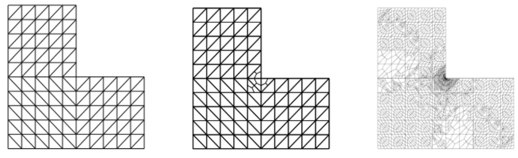
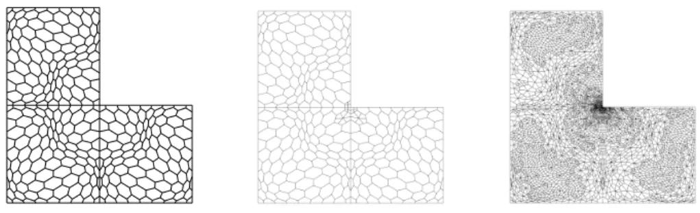
Figures 1 to 2 show the adaptively refined meshes obtained with VEM procedures and different initial meshes. Figure 1 is initiated with a mesh of triangles, while Figure 2 is initiated with a non-structured hexagonal meshes made of convex hexagons.
Figure 1. Test 1. Adaptively refined meshes obtained with VEM scheme at refine- ment steps 0, 1 and 8 (Adaptive VEM).
Figure 2. Test 1. Adaptively refined meshes obtained with VEM scheme at refine- ment steps 0, 1 and 8 (Adaptive VEM).
Figures 1 and 2 show that our estimator identifies the singularity point of the domain, leading to a refinement on the region of the re-entrant angle. This refinement allows to achieve the optimal order of convergence for the eigenvalue.
In order to compute the errors|λ1−λh1|, and since an exact eigenvalue is not known, we have used an approximation based on a least-squares fitting of the computed values obtained with extremely refined meshes. Thus, we have obtained the value λ1 = 5.9017, which has at least four accurate significant digits.
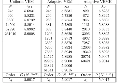
We report in Table 1 the lowest eigenvalue λh1 on uniformly refined meshes, adaptively refined meshes with VEM schemes and in the last column we report adaptively refined meshes with VEM schemes and initial non-structured hexagonal meshes. Each table includes the estimated convergence rate.
Table 1. Test 1. Computed lowest eigenvalueλh1computed with different schemes.
Uniform VEM Adaptive VEM Adaptive VEMH
N λh1 N λh1 N λh1
245 5.6831 245 5.6831 829 5.8283
940 5.8231 266 5.7356 872 5.8495
3680 5.8732 288 5.7554 945 5.8605
14560 5.8914 381 5.7805 1131 5.8688
57920 5.8982 889 5.8440 2010 5.8833
231040 5.9008 1206 5.8620 3296 5.8895
1731 5.8713 4932 5.8928
3639 5.8876 7287 5.8955
5206 5.8924 12003 5.8982
7653 5.8949 19349 5.8998
14545 5.8985 30751 5.9007 22982 5.9000 50421 5.9014 33844 5.9006
61641 5.9015 Order O N−0.79
Order O N−1.08
Order O N−1.14
λ1 5.9017 λ1 5.9017 λ1 5.9017
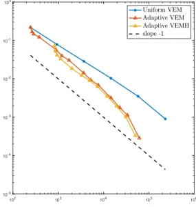
In Figure 3 we present error curves where we observe that the two refinement schemes lead to a correct convergence rate. It can be seen from Table 1 and Figure 3, that the uniform refinement leads to a convergence rate close to that predicted by the theory, while the adaptive VEM schemes allow us to recover the optimal order of convergenceO N−1
.
102 103 104 105 106 10-5
10-4 10-3 10-2 10-1 100
Figure 3. Test 1. Error curves of|λ1−λh1|for uniformly refined meshes (“Uniform VEM”), adaptively refined meshes with VEM (“Adaptive VEM”) and adaptively refined meshes with VEM and initial mesh of hexagons (“Adaptive VEMH”).
We report in Table 2, the error|λ1−λh1|and the estimatorsηat each step of the adaptive VEM scheme. We include in the table the terms θ2 := X
K∈Th
θ2K, which appears from the inconsistency of
the VEM, andJh:= X
K∈Th
X
`∈EK
hKkJ`k20,`
!
,which arise from the edge residuals. We also report in the table the effectivity indexes|λ1−λh1|/η2.
Table 2. Components of the error estimator and effectivity indexes on the adaptively refined meshes with VEM.
N λh1 |λ1−λh1| θ2 J2h η2 |λ1−λh1| η2 245 5.6831 2.1869e-01 9.4718e-03 1.3226e-01 1.4174e-01 1.5429 266 5.7356 1.6614e-01 1.2881e-02 8.5612e-02 9.8493e-02 1.6868 288 5.7554 1.4637e-01 1.2791e-02 7.5101e-02 8.7892e-02 1.6653 381 5.7805 1.2119e-01 1.2944e-02 5.6072e-02 6.9016e-02 1.7560 889 5.8440 5.7776e-02 9.4599e-03 1.5576e-02 2.5036e-02 2.3077 1206 5.8620 3.9753e-02 6.8149e-03 1.0962e-02 1.7777e-02 2.2362 1731 5.8713 3.0451e-02 5.1742e-03 8.1822e-03 1.3356e-02 2.2799 3639 5.8876 1.4166e-02 2.7744e-03 3.2286e-03 6.0030e-03 2.3598 5206 5.8924 9.3787e-03 1.8562e-03 2.3210e-03 4.1771e-03 2.2453 7653 5.8949 6.8767e-03 1.3746e-03 1.6477e-03 3.0223e-03 2.2753 14545 5.8985 3.1983e-03 7.4205e-04 9.1237e-04 1.6544e-03 1.9332 22982 5.9000 1.7633e-03 4.6344e-04 5.9698e-04 1.0604e-03 1.6628 33844 5.9006 1.1283e-03 3.3863e-04 4.2666e-04 7.6529e-04 1.4743
From Table 2 we observe that the effectivity indexes are bounded and far from zero. Also, the inconsistency and edge residual terms are, roughly speaking, of the same order. This results are
similar to those obtained in [35]. We end this test presenting in Figure 4 the displacement field and the pressure fluctuation of the fluid on the L-shaped domain, associated to the first eigenfunction.
Figure 4. Test 1. Eigenfunctions of the acoustic problem corresponding to the first lowest eigenvalue: displacement fieldwh1 (left), pressure fluctuationph1 (right).
5.2. Test 2: H-shaped domain. The aim of this test is to assess the performance of the adaptive scheme when solving a problem with a singular solution. In this test Ω consists of an H-shaped domain that represents the union of two pools. More precisely, the geometry of this domain is given by
Ω :=
(0,3/2)×(0,3) \
{[1/2,1]×[0,5/4]} ∪ {[1/2,1]×[15/8,3]} .
According to the definition of this domain, four singularities are present, leading once again to a lack of regularity for the eigenfunctions of our acoustic problem. Hence, the proposed estimatorηdefined in (24) must be capable of identify these singularities of the geometry and perform and adaptive refinement, with different polygonal meshes, in order to recover optimal order of convergence.
Figures 5 to 7 show the adaptively refined meshes obtained with VEM procedures and different initial meshes. In Figure 5 we start with a mesh of triangles and squares, while in Figure 6 we begin with a trapezoidal mesh consisting of partitions of the domain into M ×M congruent trapezoids.
Finally in Figure 7 we start with a Voronoi mesh.
Figure 5. Adaptively refined meshes obtained with VEM scheme at refinement steps 0, 1 and 8 (Adaptive VEM S-T).
Figure 6. Adaptively refined meshes obtained with VEM scheme at refinement steps 0, 1 and 8 (Adaptive VEM B).
Figure 7. Adaptively refined meshes obtained with VEM scheme at refinement steps 0, 1 and 8 (Adaptive VEM V).
Similarly to Test 1, the computations of the errors |λ2−λh2|, have been obtained with a least squares fitting of the calculated values obtained with extremely refined meshes. Thus, we have obtained the valueλ2= 1.2040, which has at least four exact significant digits.
In Table 3 we report the second lowest eigenvalue λh2 on uniformly refined meshes, adaptively refined meshes with different type of initial meshes. Each table includes the estimated convergence rate.
Table 3. Computed lowest eigenvalue λh2computed with different initial meshes.
Uniform VEM Adaptive VEM S-T Adaptive VEM B Adaptive VEM V
N λh2 N λh2 N λh2 N λh2
916 1.1831 756 1.1821 1368 1.1925 1925 1.1959
3560 1.1960 832 1.1893 1442 1.1957 2027 1.1981
14032 1.2009 1068 1.1959 1594 1.1979 2152 1.1992
55712 1.2028 1830 1.1992 1848 1.1991 2593 1.2003
222016 1.2035 3304 1.2020 2928 1.2006 3588 1.2013
4992 1.2027 5564 1.2024 6903 1.2028
8130 1.2031 8093 1.2028 9480 1.2031
16320 1.2036 12045 1.2030 12846 1.2032
23706 1.2037 21613 1.2036 15214 1.2033
Order O N−0.70
Order O N−1.19
Order O N−1.09
Order O N−1.11
λ2 1.2040 λ2 1.2040 λ2 1.2040 λ2 1.2040
In Figure 8 we present error curves where we observe that the three refinement schemes lead to a correct convergence rate. It can be seen from Table 3 and Figure 8, that the uniform refinement leads to a convergence rate close to that predicted by the theory, while the adaptive VEM schemes allow us to recover the optimal order of convergenceO N−1
.
103 104 105
10-3 10-2
Figure 8. Error curves of |λ2−λh2| for uniformly refined meshes and adaptively refined meshes VEM with different initial meshes.
In Figure 9 we present plots of the computed eigenfunctions wh2 (displacement field) and ph2
(pressure fluctuation) corresponding to the second eigenvalue.
Figure 9. Test 2. Eigenfunctions of the acoustic problem corresponding to the second lowest eigenvalue: displacement field wh2 (left), pressure fluctuation ph2
(right).
5.3. Test 3: Circular domain with obstacles. As a third test, we have considered a configuration closer to a real application: four square tubes immersed in a fluid occupying a circular cavity. Clearly in this test there are two relevant geometrical issues: in one hand, we have a non polygonal domain for which we are making an approximation by means of polygonal meshes, and the four rigid squares that lie in the interior of the circle. These tubes lead to non smooth eigenfunctions when the solutions for the acoustic problem are approximated, due the singularities of the corner on each square.
To make matters precise, let us define the circular domain by ΩC:={(x, y)∈R2 : x2+y2<1}
and the squares ΩI:= [1/5,3/5]×[1/5,3/5], ΩII:= [−3/5,−1/5]×[1/5,3/5], ΩIII:= [−3/5,−1/5]× [−3/5,−1/5] and ΩIV := [1/5,3/5]×[−3/5,−1/5]. Hence, the computational domain is Ω := ΩC\ {ΩI∪ΩII∪ΩIII∪ΩIV}.
In the sequel, we consider the fourth eigenfunction. In Figure 10 we present an adaptive refinement of our estimator when Voronoi meshes are considered. On the left hand side we present the initial mesh and, after 1 and 8 iterations of our numerical method, we observe that the estimatorηidentifies the singularities on the geometry that cause the poor regularity of the eigenfunction, and starts the refinement around these corners in order to recover the optimal order of convergence.
Figure 10. Adaptively refined meshes obtained with VEM scheme at refinement steps 0, 1 and 8 (Adaptive VEM V).
Figure 11 shows a logarithmic plot of the errors between the calculated approximations of the fourth smallest positive eigenvalue and the “exact” one, versus the number of degrees of freedom N of the meshes. As in the previous two tests, the exact value of the fourth eigenvalue is obtained by using
a least squares fit. The figure shows the results obtained with ”uniform” meshes and with adaptively refined meshes and shows how the optimal order of convergence is recovered. Finally, Figure 12 shows the eigenfunctions of the acoustic problem corresponding to the fourth lowest eigenvalue.
104 105
10-3 10-2 10-1
Figure 11. Error curves of|λ4−λh4| for uniformly refined meshes and adaptively refined meshes VEM.
Figure 12. Test 3. Eigenfunctions of the acoustic problem corresponding to the second lowest eigenvalue: displacement field wh4 (left), pressure fluctuation ph4 (right).
6. Conclusions
In this work, we have derived and analyzed an a posteriori error estimate for the acoustic vibration problem by means of mixed virtual element discretization. The theoretical analysis developed in this work was strongly supported by superconvergence results for mixed spectral formulations. Several numerical tests that substantiate the theoretical results were presented, confirming that the proposed