Augmented Fully-Mixed Finite Element Method for Coupled Flow-Transport Problems

An augmented fully-mixed finite element method for a coupled flow-transport problem

Gabriel N. Gatica^† Cristian Inzunza^‡

Abstract

In this paper we analyze the coupling of the Stokes equations with a transport problem modelled by a scalar nonlinear convection-diffusion problem, where the viscosity of the fluid and the dif- fusion coefficient depend on the solution to the transport problem and its gradient, respectively.

An augmented mixed variational formulation for both the fluid flow and the transport model is proposed. As a consequence, no discrete inf-sup conditions are required for the stability of the associated Galerkin scheme, and therefore arbitrary finite element subspaces can be used, which constitutes one of the main advantages of the present approach. In particular, the resulting fully- mixed finite element method can employ Raviart-Thomas spaces of orderkfor the Cauchy stress, continuous piecewise polynomials of degreek+ 1 for the velocity and for the scalar field, and dis- continuous piecewise polynomial approximations for the gradient of the concentration. In turn, the Lax-Milgram lemma, monotone operators theory, and the classical Schauder and Brouwer fixed point theorems are utilized to establish existence of solution of the continuous and discrete formu- lations. In addition, suitable estimates, arising from the combined use of a regularity assumption with the Sobolev embedding and Rellich-Kondrachov compactness theorems, are also required for the continuous analysis. Then, sufficiently small data allow us to prove uniqueness of solution and to derive optimal a priori error estimates. Finally, several numerical tests, illustrating the performance of our method and confirming the predicted rates of convergence, are reported.

Key words: Stokes equations, nonlinear transport problem, augmented fully–mixed formulation, fixed point theory, finite element methods, a priori error analysis

Mathematics subject classifications (2000): 65N30, 65N12, 76R05, 76D07, 65N15 35Q79, 80A20,

1 Introduction

In recent years there has been an increasing interest in studying finite element approximations to simulate the transport of a species density in an immiscible fluid. In particular, the continuous and discrete solvability of a flow-transport model given by the coupling of the Stokes equations with a scalar nonlinear convection-diffusion equation, in which the viscosity of the fluid and the effective diffusivity depend on the solution to the transport problem and its gradient, respectively, was recently analyzed in [2] by using a mixed-primal variational approach. Regarding the underlying coupled

∗This work was partially supported by CONICYT-Chile through the project AFB170001 of the PIA Program: Con- curso Apoyo a Centros Cientificos y Tecnol´ogicos de Excelencia con Financiamiento Basal; and by Centro de Investigaci´on en Ingenier´ıa Matem´atica (CI²MA), Universidad de Concepci´on.

†CI²MA and Departamento de Ingenier´ıa Matem´atica, Universidad de Concepci´on, Casilla 160-C, Concepci´on, Chile, email: [email protected].

‡CI²MA and Departamento de Ingenier´ıa Matem´atica, Universidad de Concepci´on, Casilla 160-C, Concepci´on, Chile, email: [email protected].

model, and while the original unknowns of it are the velocity of the flow, the pressure, and the local solids concentration, it is well known that other variables, such as stress tensors, vorticity, and the aforementioned gradient, are also of great interest in applications, which include natural and thermal convection, sedimentation-consolidation processes, and granular flows, among others. According to this motivation, the model is reformulated in [2] as an augmented dual-mixed formulation for the fluid flow, coupled with the usual primal method for the transport model. As a consequence, the Cauchy stress and the velocity of the fluid are sought in H(div; Ω) and H¹(Ω), respectively, whereas the concentration lies in H¹(Ω). In this way, each row of the stress tensor is approximated with Raviart- Thomas elements of order k, whereas the other two unknowns are approximated with continuous piecewise polynomials of degree ≤ k+ 1. Furthermore, fixed point arguments, suitable regularity hypotheses, the well-know Lax-Milgram theorem, classical results on monotone operators, the Sobolev embedding and Rellich-Kondrachov compactness theorems, and sufficiently small data assumptions, constitute the main tools yielding well-posedness of the continuous and Galerkin schemes, and the associated optimal a priori error estimates.

Other contributions concerning the solvability of flow-transport problems are certainly available in the literature as well. For example, the technique of parabolic regularization has been employed in [8]

for the case of large fluid viscosity, whereas the existence of solutions to a model of chemically reacting non-Newtonian fluid with the effective diffusivity depending also on the gradient of the concentration, has been established in [7]. In turn, the extension of the approach from [2] to the more realistic case of steady sedimentation-consolidation systems, in which both the viscosity and the diffusivity depend only on the scalar value of the concentration, and hence neither of them on the concentration gradient (as in [2] and [7] for the latter), was developed in [3]. In this case, the model consist in the Brinkman problem with variable viscosity, written in terms of Cauchy pseudo-stresses and bulk velocity of the mixture, coupled with a nonlinear advection – diffusion equation describing the transport of the solids volume fraction. Then, similarly to [2], the variational formulation is based on an augmented mixed approach for the Brinkman equations and the usual primal approach for the transport equation. In addition, the solvability analyses make use of basically the same arguments from [2], the finite element subspaces employed are exactly those from [2], and suitable Strang-type inequalities are utilized to derive optimal error estimates in the natural norms.

On the other hand, it is worth mentioning that flow-transport models, and specially those in- volving sedimentation-consolidation processes, share some analytical similarities with Boussinesq and related problems, for which several mixed-primal and fully-mixed formulations have been proposed in recent years (see, e.g. [11], [12], [13], [15], [16], and [24]). In particular, the mixed finite element method for the Boussinesq problem developed in [15] introduces the gradient of velocity as an aux- iliary unknown. In turn, following [9], the approach from [11] employs the nonlinear pseudostress tensor linking the pseudostress and the convective term, and then augment the resulting mixed for- mulation of the stationary Boussinesq problem with suitable Galerkin type terms. Furthermore, the technique of [12] proceeds similarly to [11], but in contrast to the latter, an augmented mixed formu- lation for the equation modelling the temperature is also proposed. More precisely, a new auxiliary vector unknown, involving the temperature, its gradient and the velocity, is introduced, and then the resulting new mixed formulation for the convection–diffusion equation is augmented with alternative testings of the constitutive and equilibrium temperature equations. In this way, classical fixed point theorems, together with the Lax-Milgram lemma and the Babuˇska-Brezzi theory, are applied to prove the well-posedness of the continuous and discrete formulations in [11] and [12]. However, up to our knowledge, fully-mixed formulations specifically designed for flow-transport models, and aiming to introduce further unknows of physical interest, are not yet available in the literature.

According to the previous bibliographic discussion, the purpose of the present paper is to keep contributing in the direction of [2] and [3] by applying now an augmented mixed variational formulation to both the fluid flow and the transport model. In this way, and besides the incorporation of other

unknowns of physical interest, such as the gradient of concentration, the resulting decoupled problems yield a strongly elliptic bilinear form and a strongly monotone operator equation, respectively, and hence arbitrary finite element subspaces can be employed for defining the associated discrete schemes.

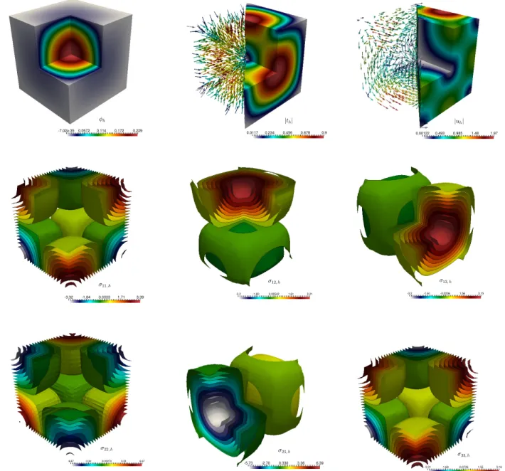
The contents of the paper are organized as follows. The remainder of this section introduces some standard notation and functional spaces. In Section2 we first describe the boundary value problem of interest, then slightly simplify it by eliminating the pressure unknown in the fluid and defining the gradient of the concentration as a new unknown variable. Next, in Section3we introduce and analyze the continuous formulation, which is defined by an augmented mixed approach in both media. The necessity of augmentation is clearly justified, and the solvability analysis is based on a fixed point strategy that makes use of the Lax-Milgran lemma, the Schauder theorem, and a well-known result on strongly monotone operators. We prove existence of solution and for sufficiently small data we derive uniqueness. The associated Galerkin scheme is introduced in Section4 by employing Raviart- Thomas elements for the stress, continuous piecewise polynomial approximations for the velocity and concentration, and discontinuous piecewise polynomial approximations for the gradient of the concentration. Here the solvability is established by applying now the Brouwer fixed point theorem and analogue arguments to those employed in Section 3. In Section 5 we assume again sufficiently small data and, using a suitable Strang-type estimate for nonlinear problems, provide optimal a priori error estimates. Finally, in Section6we present numerical examples illustrating the good performance of the fully-mixed method and confirming the theoretical rates of convergence.

Preliminary notations

Let Ω ⊆ Rⁿ, n = 2,3, be a given bounded domain with polyhedral boundary Γ = ¯Γ_D ∪Γ¯_N, with

|Γ_D|,|Γ_N| > 0, ΓD ∩ΓN = ∅ and denote by ν the outward unit normal vector on Γ. A standard notation will be adopted for Lebesgue spaces L^p(Ω) and Sobolev spaces H^s(Ω) with norm k · k_s,Ω and seminorm | · |_s,Ω. In particular, H^1/2(Γ) is the space of traces of functions of H¹(Ω) and H^−1/2(Γ) denotes its dual. In addition, given Γ∗ ⊆ Γ with ∗ ∈ {D, N}, denote by h·,·i_Γ∗ the duality pairing between H^1/2(Γ∗) and H^−1/2(Γ∗). Also, we let Mand M be the vectorial and tensorial counterparts of a generic scalar functional space M. In turn, I stands for the identity tensor in R^n×n, and | · | denotes both the euclidean norm in Rⁿ and the Frobenius norm in R^n×n. On the other hand, for any vector field υ = (vi)i=1,n we set ∇υ :=

∂v_i

∂xj

i,j=1,n and divυ :=

n

X

j=1

∂v_j

∂xj

. Additionaly, for any tensor fields τ = (τi,j)i,j=1,n and ζ = (ζij)i,j=1,n, we let divτ be the divergence operator div acting along the rows ofτ, and define the transpose, the trace, the tensor product, and the deviatoric tensor, respectively, as

τ^t := (τji)i,j=1,n, tr(τ) :=

n

X

i=1

τii, τ :ζ :=

n

X

i,j=1

τijζij and τ^d :=τ −1

ntr(τ)I. Furthermore, we recall that the space

H(div,Ω) :=

n

τ ∈L²(Ω) : divτ ∈L²(Ω) o

,

equipped with the usual norm kτk²_div;Ω:=kτk²_0,Ω+kdivτk²_0,Ω, is a Hilbert space.

2 The model problem

The following system of partial differential equations, written as to apply a fully-mixed approach, describes the stationary state of the transport of species in an immiscible fluid occupying the domain Ω⊆Rⁿ:

σ = µ(φ)∇u−pI, in Ω,

−divσ = fφ, in Ω,

div u = 0 in Ω,

p = θ(|∇φ|)∇φ−φu−γ(φ)k in Ω,

div p = −g in Ω,

u = u_D on Γ_D,

σν = 0 on ΓN,

φ = φ_D on Γ_D,

p·ν = 0 on Γ_N,

(2.1)

where the sought quantities are the Cauchy fluid stress σ, the local volume-average velocity of the fluidu, the pressurep, and the local concentration of species φ. Regarding this study, we will restrict ourselves to a specific physical scenario corresponding to the process of sedimentation-consolidation of a mixture. Also, µ : R⁺ → R⁺ is the kinematic effective viscosity, θ : R⁺ → R⁺ is the diffusion term modelling e.g. sediment compressibility, and γ : R⁺ →R is the one dimensional flux describing hindered settling, all them nonlinear functions. In addition, k is a constant vector pointing in the direction of gravity, and f ∈ L^∞(Ω), g ∈ L²(Ω), uD ∈ H^1/2(ΓD) and φD ∈ H^1/2(ΓD) are given functions. We assume that:

i) there existµ1,µ2,γ1,γ2 >0 such that

µ₁ ≤µ(φ)≤µ₂ and γ₁≤γ(φ)≤γ₂ ∀φ∈R⁺, (2.2) ii) θ∈C¹(R⁺) and there existθ1, θ2>0 such that

θ1≤θ(s)≤θ2 and θ1 ≤θ(s) +sθ⁰(s)≤θ2 ∀s∈R⁺, (2.3) iii) there exist L_µ, L_γ>0 such that

|µ(s)−µ(t)| ≤Lµ|s−t| and |γ(s)−γ(t)| ≤Lγ|s−t| ∀s, t ∈R⁺. (2.4) Now, following the approach employed in [2] y [3] , it can be seen from the first and third equations of (2.1) that

p=−1

n tr (σ) inΩ, (2.5)

which allows us to eliminate the pressure. Next, introducing the auxiliary unknownt:=∇φin Ω, the fourth equation of (2.1) is rewritten as

p=θ(|t|)t−φu−γ(φ)k in Ω, and hence, the coupled problem (2.1) becomes

1

µ₍φ)σ^d = ∇u in Ω,

−divσ = fφ, in Ω,

t = ∇φ in Ω,

p = θ(|t|)t−φu−γ(φ)k in Ω,

div p = −g in Ω,

u = u_D on Γ_D,

σν = 0 on Γ_N,

φ = φD on ΓD,

p·ν = 0 on Γ_N.

(2.6)

We remark here that the incompressibility constraint divu = 0 ∈ Ω is implicitly present in the first equation of (2.6), that is in the constitutive equation relatingσand u. Also, we observe that the pressure can be approximated later on through the post-process suggested by (2.5).

3 The continuous formulation

3.1 The augmented fully-mixed formulation

We begin by observing that the homogeneous Neumann boundary conditions for σ and p in ΓN

suggest the introduction of the following spaces HN(div,Ω) :=n

τ ∈H(div,Ω) : τ ν =0 on Γ_No , H_N(div,Ω) :=n

q∈H(div,Ω) : q·ν = 0 on Γ_No .

Then, multiplying the first equation of (2.6) by τ ∈HN(div,Ω), integrating by parts, and using the Dirichlet boundary condition foru, we obtain

Z

Ω

1

µ(φ)σ^d:τ^d+ Z

Ω

u·divτ =hτ ν,u_Di_ΓD ∀τ ∈HN(div,Ω). (3.1) In addition, the equilibrium equation, that is the second equation of (2.6), is rewritten as

Z

Ω

υ·divσ=− Z

Ω

fφ·υ ∀υ∈L²(Ω). (3.2)

Similarly for deriving the weak formulation of the transport equation we multiply byq∈H_N(div,Ω) the third equation of (2.6), integrate by parts, and use the Dirichlet boundary condition forφ, to yield

Z

Ω

t·q+ Z

Ω

φdivq=hq·ν, φDi_ΓD ∀q∈HN(div,Ω). (3.3) Also, the corresponding equilibrium equation is stated as

Z

Ω

ϕdivp=− Z

Ω

g ϕ ∀ϕ∈L²(Ω). (3.4)

Finally, multiplying by s∈L²(Ω) the fourth equation of (2.1) and integrating, we arrive at Z

Ω

θ(|t|)t·s− Z

Ω

p·s− Z

Ω

φu·s= Z

Ω

γ(φ)k·s ∀s∈L²(Ω). (3.5) Summarizing, given φ ∈ L²(Ω), we obtain form (3.1) and (3.2) the following mixed formulation for the flow equations: Find (σ,u)∈HN(div,Ω)×L²(Ω) such that

a_φ(σ,τ) +b(τ,u) = hτ ν,u_Di_ΓD ∀τ ∈HN(div,Ω), b(σ,υ) = −

Z

Ω

fφ·υ ∀υ ∈L²(Ω), (3.6)

whereaφ:HN(div,Ω)×HN(div,Ω)→R andb:HN(div,Ω)×L²(Ω)→R are the bounded bilinear forms defined by

a_φ(ζ,τ) :=

Z

Ω

1

µ(φ)ζ^d:τ^d and b(τ,υ) :=

Z

Ω

υ·divτ,

forζ,τ ∈HN(div,Ω) and υ∈L²(Ω).

In turn, given u ∈ L²(Ω), at first instance we get from (3.3), (3.4) and (3.5) the following mixed formulation for the transport equations: Find (t,p, φ)∈L²(Ω)×H_N(div,Ω)×L²(Ω) such that

Z

Ω

t·q+ Z

Ω

φdivq = hq·ν, φDi_ΓD ∀q∈HN(div,Ω), Z

Ω

θ(|t|)t·s− Z

Ω

p·s− Z

Ω

φu·s = Z

Ω

γ(φ)k·s ∀s∈L²(Ω), Z

Ω

ϕdivp = − Z

Ω

g ϕ ∀ϕ∈L²(Ω).

(3.7)

Then, we observe that the assumption on µgiven by (2.2) and the Babuska-Brezzi theory suffice to show that (3.6) is well-possed (see, e.g. [18, Thm. 2.1] for details). However, in order to deal with the analysis of (3.7), particularly to handle the third term of the second equation, it is required that actuallyuand φbelong to H¹(Ω) and H¹(Ω) respectively. In fact, using Cauchy-Schwarz’s inequality and the continuous injectionsi: H¹(Ω)→L⁴(Ω) and i:H¹(Ω)→L⁴(Ω), we have that

Z

Ω

ϕυ·s

≤c(Ω)kυk_1,Ωkϕk_1,Ωksk_0,Ω ∀(υ, ϕ,s)∈H¹(Ω)×H¹(Ω)×L²(Ω), (3.8) withc(Ω) :=kik kik. Furthermore, while the exact solutions of (3.6) and (3.7) satisfy 1

µ₍φ)σ^d =∇u in D⁰(Ω) and t =∇φ in D⁰(Ω), which implies that u ∈H¹(Ω) and φ∈ H¹(Ω), these distributional identities do not necessarily extend to the discrete cases of (3.6) and (3.7). Therefore, proceeding as in [2], we now incorporate the following redundant Galerkin terms

k1

Z

Ω

∇u− 1 µ(φ)σ^d

:∇υ = 0 ∀υ ∈ H¹(Ω),

k₂ Z

Ω

divσ·divτ = −k₂ Z

Ω

fφ·divτ ∀τ ∈ HN(div,Ω), k3

Z

ΓD

u·υ = k3

Z

ΓD

uD·υ ∀υ ∈ H¹(Ω),

(3.9)

where (k₁, k₂, k₃) is a vector of positive parameters to be specified later on. Notice that the first and third equations in (3.9) implicitly require the velocity u to belong to H¹(Ω). In this way, instead of (3.6), from now on we consider the following augmented mixed formulation: Find (σ,u) ∈H1 :=

HN(div,Ω)×H¹(Ω) such that

B_φ((σ,u),(τ,υ)) =F_φ(τ,υ) ∀(τ,υ)∈H1, (3.10) where

B_φ((σ,u),(τ,υ)) := a_φ(σ,τ) +b(τ,u)−b(σ,υ) +k₁ Z

Ω

∇u− 1 µ(φ)σ^d

:∇υ + k₂

Z

Ω

divσ·divτ+k₃ Z

ΓD

u·υ

(3.11)

and

F_φ(τ,υ) := hτ,u_Di_ΓD + Z

Ω

fφ·υ−k₂ Z

Ω

fφ·divτ+k₃ Z

ΓD

u_D·υ. (3.12)

Similarly, the transport formulation (3.7) is augmented with the following redundant Galerkin terms l₁

Z

Ω

(p−θ(|t|)t+φu)·q = −l₁ Z

Ω

γ(φ)k·q ∀q ∈ H_N(div,Ω), l2

Z

Ω

divpdivq = −l₂ Z

Ω

gdivq ∀q ∈ HN(div,Ω), l₃

Z

Ω

(∇φ−t)· ∇ϕ = 0 ∀ϕ ∈ H¹(Ω),

l4

Z

Γ_D

φϕ = l4

Z

Γ_D

φDϕ ∀ϕ ∈ H¹(Ω),

(3.13)

where (l1, l2, l3, l4) is a vector of positive parameters to be specified later on. Analogously as before, the third and fourth equations of (3.13) require that φ belongs to H¹(Ω). In this way, instead of (3.7), we consider from now on the following augmented mixed formulation: Find (t,p, φ) ∈ H₂ :=

L²(Ω)×HN(div,Ω)×H¹(Ω) such that

[(A+Be_u)(t,p, φ),(s,q, ϕ)] = Fe_φ(s,q, ϕ) ∀(s,q, ϕ)∈L²(Ω)×H_N(div,Ω)×H¹(Ω) (3.14) where [·,·] stands for the duality pairing between H2 and H₂⁰, A :H₂⁰ → H2 and Beu : H₂⁰ → H2 are the nonlinear and linear operators, respectively, given by

[A(t,p, φ),(s,q, ϕ)] :=

Z

Ω

θ(|t|)t·s− Z

Ω

p·s+ Z

Ω

t·q+ Z

Ω

φdivq− Z

Ω

ϕdivp +l1

Z

Ω

(p−θ(|t|)t)·q+l2

Z

Ω

divpdivq+l3

Z

Ω

(∇φ−t)· ∇ϕ+l4

Z

ΓD

φϕ ,

(3.15)

and

[Beu(t,p, φ),(s,q, ϕ)] :=

Z

Ω

φu·(l1q−s), (3.16)

and Fe_φ∈H₂⁰ is defined by

Fe_φ(s,q, ϕ) :=hq·ν, φ_Di_ΓD+ Z

Ω

γ(φ)k·(s−l₁q) + Z

Ω

ϕ g−l₂ Z

Ω

gdivq+l₄ Z

ΓD

φ_Dϕ (3.17) for all (s,q, ϕ) ∈H₂. The well-posedness of (3.10) and (3.14) is proved below in Section 3.3. Con- sequently, the augmented fully mixed formulation of the coupled problem (2.6) reduces to: Find ((σ,u,),(t,p, φ))∈H1×H2 such that

Bφ((σ,u),(τ,υ)) = Fφ(τ,υ) ∀(τ,υ)∈H1, h

(A+Beu)(t,p, φ),(s,q, ϕ) i

= Feφ(s,q, ϕ) ∀(s,q, ϕ)∈H2. (3.18) 3.2 A fixed point strategy

According to the alternative formulations (3.10) and (3.14), and proceeding as in [2] and [3] (se also, [11] and [12]), we suggest a fixed point strategy to analyze (3.18). Indeed, letS: H¹(Ω)→H1 be the operator defined by

S(ψ) = (S1(ψ),S2(ψ)) := (σ,u) ∈H1 ∀ψ∈H¹(Ω),

where (σ,u) is the unique solution of (3.10) with the givenφ=ψ. In turn, letSe : H¹(Ω)×H¹(Ω)→H₂ be the operator defined by

S(ψ,e u) = (eS₁(ψ,u),Se₂(ψ,u),Se₃(ψ,u)) := (t,p, φ)∈H₂,

where (t,p, φ) is the unique solution of (3.14) withφ=ψ and ugiven. Then, we define the operator T: H¹(Ω)→H¹(Ω) by

T(ψ) :=eS3(ψ,S2(ψ)) (3.19) and realize that solving (3.18) is equivalent to seeking a fixed point of T, that is : Find ψ ∈ H¹(Ω) such that

T(ψ) =ψ . (3.20)

3.3 Well-posedness of the uncoupled problems

In this section, we show that the operators S and Se are well defined, that is that the uncoupled problems (3.10) and (3.14) are in fact well-posed. We begin by recalling (see, e.g. [6]) that

H(div,Ω) =H0(div,Ω)⊕RI, where H0(div,Ω) :=n

ζ ∈H(div,Ω) : Z

Ω

tr (ζ) = 0o . More precisely, for each ζ ∈ H(div,Ω) there exists unique ζ₀ := ζ−n 1

n|Ω|

Z

Ω

tr (ζ)o

I ∈ H0(div,Ω) andd:= 1

n|Ω|

Z

Ω

tr (ζ)∈R such thatζ =ζ₀+dI. The following three lemmas from [6], [19] and [17], which concern the above decomposition and an equivalence of norm, will be employed to show the well-posedness of (3.10) and (3.14).

Lemma 3.1. There exists c₁ =c₁(Ω)>0 such that

c₁kτ₀k²_0,Ω≤ kτ^dk²_0,Ω+kdiv(τ)k²_0,Ω ∀τ = τ₀+cI ∈ H(div,Ω), withτ₀ ∈H0(div,Ω) and c∈R.

Proof. See [6, Proposition 3.1].

Lemma 3.2. There exists c2 =c2(Ω,ΓN)>0) such that

c2kτk²_div;Ω≤ kτ₀k²_div;Ω ∀τ =τ0+cI ∈ HN(div,Ω) withτ₀ ∈ H0(div,Ω) and c ∈ R.

Proof. See [19, Lemma 2.2].

Lemma 3.3. There exists c_i =c_i(Ω, γ_D)>0 , withi∈ {3,4} such that

|υ|²_1,Ω+kυk²_0,Γ

D ≥c3kυk²_1,Ω ∀υ∈ H¹(Ω)

|ϕ|²_1,Ω+kϕk²_0,Γ

D ≥c4kϕk²_1,Ω ∀ϕ ∈ H¹(Ω) Proof. It corresponds to a slight modification of the proof of [17, Lemma 3.3].

On the other hand, the following results refers to the nonlinear term forming part ofA(cf. (3.15)).

Lemma 3.4. Let θe₂ :=max{θ₂,2θ₂−θ₁} (cf. (2.3)). Then

kθ(|r|)r−θ(|s|)sk_0,Ω ≤θe₂kr−sk_0,Ω Z

Ω

{θ(|r|)r−θ(|s|)s} ·(r−s)≥θ₁kr−sk_0,Ω² for allr,s ∈ L²(Ω).

Proof. See [20, Theorem 3.8] for details.

In what follows, we consider k(τ,υ)k_H1 :=

n

kσk²_div;Ω+kυk²_1,Ωo1/2

∀(τ,υ)∈H1

and

k(s,q, ϕ)k_H2 :=n

ksk²_0,Ω+kqk²_div;Ω+kϕk²_1,Ωo1/2

∀(s,q, ϕ)∈H₂. We now prove the well-definiteness of S.

Lemma 3.5. Assume that k1 ∈

0,2δµ₁ µ2

with δ ∈ (0,2µ1), and that 0 < k2, k3. Then, for each φ ∈ H¹(Ω) the problem (3.10) has a unique solution S(φ) := (σ,u) ∈ H₁. Moreover, there exists CS > 0, independent of φ, such that

kS(φ)k_H1 = k(σ,u)k_H1 ≤CS

n

ku_Dk_1/2,ΓD+kfk∞,Ωkφk_1,Ωo

∀φ ∈ H¹(Ω). (3.21) Proof. It reduces to show that, under the stipulated ranges for the parameters κ1,κ2,κ3, andδ, the bilinear formB_φbecomesH₁-elliptic with an ellipticity constant independent ofφ∈H¹(Ω). We omit details and refer to [2, Lemma 3.4].

Throughout the rest of the paper, a regularity assumption will be made for the problem defining the operatorS. More precisely, we assume that u_D ∈H^1/2+ε for some

ε∈

(0,1) if n= 2,

(¹₂,1) if n= 3, (3.22)

and that for eachφ∈H¹(Ω) withkφk_1,Ω ≤r,r >0, there holdsS(φ) = (ζ,s)∈(HN(div,Ω)∩H^ε(ε))

× H¹(Ω)∩H^1+ε(Ω) and

kζk_ε,Ω+ksk_1+ε,Ω ≤Ce

eS(r)n

ku_Dk_1/2+ε,Γ

D+kfk_∞,Ωkφk_0,Ωo

, (3.23)

with a positive constantCe

eS(r) independent of the givenφbut depending on the upper boundr of its H¹-norm. We remark that the reason of the stipulated ranges forεwill be clarified in the forthcoming analysis (see below proof of Lemma3.11). For more details see [2].

Next, in order to demonstrate that S is well-posed, we need the following two previous Lemmas.

Lemma 3.6. For each u∈H¹(Ω), A+Be_u is Lipschitz-continuous.

Proof. Given (t,p, φ),(r,o, ψ) and (s,q, ϕ)∈H₂, we first notice that

[A(t,p, φ) − A(r,o, ψ),(s,q, ϕ)]

= Z

Ω

{θ(|t|)t−θ(|r|)r} ·s+ Z

Ω

(o−p)·s+ Z

Ω

(t−r)·q

+ Z

Ω

(φ−ψ)·q+ Z

Ω

ϕdiv (o−p) +l1

Z

Ω

(o−p)·q+l1

Z

Ω

{θ(|t|)t−θ(|r|)r} ·q

+ l₂ Z

Ω

div (p−q) divq+l₃ Z

Ω

∇(φ−ψ)· ∇ϕ+l₃ Z

Ω

(r−t)· ∇ϕ+l₄ Z

ΓD

(φ−ψ)ϕ

Now, using the Cauchy-Schwarz inequality, the Lipschitz-continuity of the operator induced byθ(cf.

Lemma3.4) and the trace theorem (with constantc₀ ), we deduce from the foregoing equation that

[A(t,p, φ)−A(r,o, ψ),(s,q, ϕ)]

≤ kθ(|t|)t−θ(|r|)rk_0,Ωksk_0,Ω+ko−pk_0,Ωksk_0,Ω +kt−rk_0,Ωkqk_0,Ω+kφ−ψk_0,Ωkqk_0,Ω+kϕk_0,Ωkdiv (o−p)k_0,Ω

+l₁ko−pk_0,Ωkqk_0,Ω+l₁kθ(|t|)t−θ(|r|)rk_0,Ωkqk_0,Ω+l₂kdiv (p−q)k_0,Ωkdivqk_0,Ω +l₃|φ−ψ|_1,Ω|ϕ|_1,Ω+l₃kr−tk_0,Ω|ϕ|_1,Ω+l₄kφ−ψk_0,ΓDkϕk_0,ΓD

≤Le_A(4kt−rk²_0,Ω+ 2kp−ok²_0,Ω+ 2kφ−ψk²_1,Ω

+ 2kdiv (p−o)k²_0,Ω+|φ−ψ|²_1,Ω)^1/2(2ksk²_0,Ω+ 4kqk²_0,Ω+kϕk²_0,Ω+kdivqk²_0,Ω + 2|ϕ|²_1,Ω+kϕk²_1,Ω)^1/2,

withLe_A= max{eθ₂,1, l₁, l₁eθ₂, l₂, l₃, l₄c₀}, which yields [A(t,p, φ)−A(r,o, ψ),(s,q, ϕ)]

≤L_Ak(t,p, φ)−(r,o, ψ)k_H2k(s,q, ϕ)k_H2 (3.24) for all (t,p, φ),(r,o, ψ),(s,q, ϕ) ∈ H2, with LA := 4LeA. In turn, it readily follows from (3.8) and (3.16) that

|[Beu(s,q, ϕ),(r,o, ψ)]|=

Z

Ω

ϕu·(l1o−r)

≤ kϕk_L4(Ω)kuk_L4(Ω)(l²₁+ 1)^1/2n

krk²_0,Ω+kok²_div;Ωo1/2

≤c(Ω)(l²₂+ 1)^1/2kuk_1,Ωkϕk_1,Ωk(r,o, ψ)k_H2

≤c(Ω)(l²₂+ 1)^1/2kuk_1,Ωk(s,q, ϕ)k_H2k(r,o, ψ)k_H2,

(3.25)

which, thanks to the linearity of Be_u, and together with (3.24), confirms that A+Be_u is Lipschitz- continuous with constantLC :=LA+c(Ω)(l₂²+ 1)^1/2kuk_1,Ω.

The strong monotonicity of the operator A+Be_u is established next.

Lemma 3.7. Assume thatl₁ ∈ 0,^2θ1δ

θe2

and l₃ ∈ 0,2eδ θ₁−^eθ_2δ^2l1)

, withδ ∈ 0, ²

θe2

and eδ∈(0,2), and thatl₂, l₄ >0. Then, for each u∈H¹(Ω)such thatkuk_1,Ω≤ α(Ω)

2c(Ω)(1 +l²₁)^1/2, A+Be_u is strongly monotone.

Proof. Given (s,q, ϕ),(r,o, ψ)∈H2, we first observe that [A(s,q, ϕ)−A(r,o, ψ),(s,q, ϕ)−(r,o, ψ)] =

Z

Ω

nθ(|s|)s−θ(|r|)ro

·(s−r) +l₁kq−ok²_0,Ω

−l₁ Z

Ω

(θ(|s|)s−θ(|r|)r)·(q−o) +l2kdiv(q−o)k²_0,Ω+l3|ϕ−ψ|²_1,Ω

−l₃ Z

Ω

(s−r)· ∇(ϕ−ψ) +l₄kϕ−ψk²_0,Γ

D.

Then, thanks to Lemma3.4and the Cauchy-Schwarz and Young inequalities, we obtain

[A(s,q, ϕ)−A(r,o, ψ),(s,q, ϕ)−(r,o, ψ)]≥θ1ks−rk²_0,Ω+l1kq−ok²_0,Ω+l2kdiv (q−o)k²_0,Ω

−l₁kθ(|s|)s−θ(|r|)rk_0,Ωkq−ok_0,Ω+l₃|ϕ−ψ|²_1,Ω−l₃ks−rk_0,Ω|ϕ−ψ|_1,Ω+l₄kϕ−ψk_0,ΓD

≥θ₁ks−rk²_0,Ω+l₁kq−ok²_0,Ω−l₁θe₂ks−rk_0,Ωkq−ok_0,Ω+l₂kdiv (q−o)k²_0,Ω+l₃|ϕ−ψ|²_1,Ω

−l3ks−rk_0,Ω|ϕ−ψ|_1,Ω+l4kϕ−ψk_0,ΓD

≥θ₁ks−rk²_0,Ω+l₁kq−ok²_0,Ω−l₁θe₂ 1

2δks−rk²_0,Ω−l₁θe₂δ

2kq−ok²_0,Ω+l₂kdiv (q−o)k²_0,Ω +l3|ϕ−ψ|²_1,Ω−l3

1

2eδks−rk²_0,Ω−l3

eδ

2|ϕ−ψ|²_1,Ω+l4kϕ−ψk_0,ΓD, which gives

[A(s,q, ϕ)−A(r,o, ψ),(s,q, ϕ)−(r,o, ψ)]≥

θ₁−l₁θe_22δ¹ −l₃ ¹

2eδ

ks−rk²_0,Ω +l1

1− ^eθ2₂^δ

kq−ok²_0,Ω+l2kdiv (q−o)k²_0,Ω+l3

1−^eδ₂

|ϕ−ψ|²_1,Ω+l4kϕ−ψk_0,ΓD (3.26) In this way, assuming the stipulated hypotheses onδ, l1, l2, l3, l4, we can define the positive constants

α₀(Ω) :=

θ₁−l₁θe₂ 1

2δ −l₃ 1 2eδ

, α₁(Ω) := minn l₁

1−θe₂δ 2

, l₂o

, and

α₂(Ω) := minn l₃

1−δe 2

, l₄o , which, together with (3.26), imply that

[A(s,q, ϕ)−A(r,o, ψ),(s,q, ϕ)−(r,o, ψ)]≥α(Ω)k(s,q, ϕ)−(r,o, ψ)k²_H

2, (3.27) with

α(Ω) := min n

α0(Ω), α1(Ω), c4α2(Ω) o

. (3.28)

Moreover, by combining (3.25) and (3.27), we obtain

[(A+Be_u)(s,q, ϕ)−(A+Be_u)(r,o, ψ),(s,q, ϕ)−(r,o, ψ)]

≥n

α(Ω)−(1 +l²₁)^1/2c(Ω)kuk_1,Ωo

k(s,q, ϕ)−(r,o, ψ)k²_H

2,

(3.29)

and assuming thatkuk_1,Ω≤ α(Ω)

2c(Ω)(1 +l²₁)^1/2 we conclude that [(A+Beu)(s,q, ϕ)−(A+Beu)(r,o, ψ),(s,q, ϕ)−(r,o, ψ)]≥ α(Ω)

2 k(s,q, ϕ)−(r,o, ψ)k²_H

2, (3.30) which shows the strong monotonicity of A+Be_u with constant ^α(Ω)₂ .

Having proved the properties ofA+Be_u given by the previous Lemmas3.6and 3.7, we are now in a position to show the well-posedness of the operatoreS.

Lemma 3.8. Assume thatl₁ ∈ 0,^2θ1δ

θe2

and l₃ ∈ 0,2eδ θ₁−^eθ_2δ^2l1)

, withδ ∈ 0, ²

θe2

and eδ∈(0,2), and that l2, l4 >0. Then given φ∈H¹(Ω)and u∈H¹(Ω)such that kuk_1,Ω ≤ α(Ω)

2c(Ω)(1 +l₁²)^1/2, there exists a uniqueS(φ,e u) := (t,p, φ)∈H₂ solution of (3.14) and there hols

keS(φ,u)k_H2 =k(t,p, φ)k_H2 ≤C

Se

n

kφ_Dk_1/2,ΓD + 2kkk+ 2kgk_0,Ω+kφ_Dk_0,ΓDo

, (3.31)

where C

eS= 2 α(Ω)C

Feφ and C

Feφ = maxn

1, γ₂|Ω|^1/2kkk, γ₂|Ω|^1/2kkkl₁, l₂, c₀l₄o .

Proof. Given φ ∈ H¹(Ω), we begin by noticing that the Cauchy-Schwarz inequality and the trace theorems imply

|Feφ(s,q, ϕ)| ≤ |hq·ν, φDi_ΓD|+ Z

Ω

γ(φ)k·(s−l1q)

+ Z

Ω

ϕg

+l2

Z

Ω

gdivq

+l4

Z

ΓD

φDϕ

≤ kqk_−1/2,ΓDkφ_Dk_1/2,ΓD+γ2|Ω|^1/2kkkks−l1qk_0,Ω+kgk_0,Ωkϕk_0,Ω + l₂kgk_0,Ωkdivqk_0,Ω+l₄kφ_Dk_0,ΓDkϕk_0,ΓD

≤ kqk_{div ;Ω}kφ_Dk_1/2,Γ

D+γ₂|Ω|^1/2kkk(ksk_0,Ω+l₁kqk_{div ;Ω}) +kgk_0,Ωkϕk_1,Ω + l2kgk_0,Ωkqk_{div ;Ω}+l4c0kφ_Dk_0,ΓDkϕk_1,Ω

≤ C_Fe

φ

n

kφ_Dk_1/2,ΓD+ 2kkk+ 2kgk_0,Ω+kφ_Dk_0,ΓDo

k(s,q, ϕ)k_H2,

(3.32) with C

Feφ = maxn

1, γ₂|Ω|^1/2kkk, γ₂|Ω|^1/2kkkl₁, l₂, c₀l₄o

, which shows that Fe_φ ∈ H₂⁰. In this way, knowing from Lemmas3.6and3.7that for eachu∈H¹(Ω) the operatorA+Beuis Lipschitz-continuous and strongly monotone, a classical result on the bijectivity of monotone operators (see e.g. [23, Theorem 3.3.23]) allows us to conclude that there exists a unique solutioneS(φ,u) := (t,p, φ)∈H₂ of (3.14). Then, by applying (3.30) with (s,q, ϕ) = (t,p, φ) and (r,o, ψ) = (0,0,0), we obtain

α(Ω)

2 k(t,p, φ)k²_H

2 ≤[(A+Beu)(t,p, φ),(t,p, φ)]≤ |Fe_φ(t,p, φ)|

≤C

Feφ

n

kφ_Dk_1/2,ΓD+ 2kkk+ 2kgk_0,Ω+kφ_Dk_0,ΓDo

k(t,p, φ)k_H2, which yields

k(t,p, φ)k_H2 ≤C

Se

n

kφ_Dk_1/2,ΓD+ 2kkk+ 2kgk_0,Ω+kφ_Dk_0,ΓDo .

We end this section by remarking that a suitable constant α0(Ω) can be computed by taking the parametersδ, l1,eδandl3 as the middle points of their feasible ranges. Then we choosel2 andl4 so that the minima definingα₁(Ω) andα₂(Ω) are maximized. More precisely, we simply takeδ= 1

θe2

andeδ = 1, which impliesl1 = θ1

θe²₂, and l3 = θ1

2 , and then we setl2=l1

1− θe2δ 2

= ^l₂¹, and l4=l3

1− eδ

2

= ^l₂³, whence

α0(Ω) =

θ1−l1θe2

1 2δ −l3

1 2eδ

= θ₁ 2 ,

α1(Ω) = min{l₁

1−θe2δ 2

, l2}= l1

2 = θ1

4eθ²₂ , α₂(Ω) = min{l₃

1−eδ 2

, l₄}= l₃ 2 = θ₁

4 , and

α(Ω) = min n

α0(Ω), α1(Ω), c4α2(Ω) o

= min nθ1

2, θ1

4θe₂², c4

θ1

4 o

.

The foregoing explicit values of the stabilization parameters l_i, i ∈ {1, ...,4}, will be employed in Section 5 for the corresponding numerical experiments.

3.4 Solvability analysis of the fixed point equation

Having established in the previous section the well-posedness of the uncoupled problems (3.10) and (3.14), thus showing that the operators S,eS and T are well defined, we now address the solvability analysis of the fixed point equation (3.20). For this purpose, in what follows we verify the hypotheses of the Schauder fixed point theorem, which is recalled next (cf. [10, Theorem. 9.12-1(b)]).

Theorem 3.9. Let W be a closed and convex subset of a Banach space X and letT:W →W be a continuous mapping such that T(W) is compact. Then T has at least one fixed point.

We start with the following result.

Lemma 3.10. Givenr >0, set W:=n

φ∈H¹(Ω) :kφk_1,Ω≤ro

, and assume that the data satisfy C_S

n

ku_Dk_1/2,ΓD +rkfk_∞,Ωo

≤ α(Ω)

2c(Ω)(1 +l²₁)^1/2 (3.33) and

CSe

n

kφ_Dk_1/2,ΓD+ 2kkk+ 2kgk_0,Ω+kφ_Dk_0,ΓDo

≤r . (3.34)

ThenT(W)⊆W.

Proof. Givenφ∈W, we get from (3.21) (cf. Lemma 3.5) that kS(φ)k_H1 = k(σ,u)k_H1 ≤C_Sn

ku_Dk_1/2,Γ

D +kfk_∞,Ωkφk_1,Ωo

and hence, thanks to the restriction (3.33), we observe that u = S2(φ) satisfies the assumption requested in the statement of Lemma3.8. Moreover, the corresponding estimate (3.31) gives

kT(φ)k_1,Ω=keS3(φ,u)k_1,Ω≤ keS(φ,u)k_H2 =k(t,p, φ)k_H1

≤C

Se

n

kφ_Dk_1/2,ΓD + 2kkk+ 2kgk_0,Ω+kφ_Dk_0,ΓDo ,

(3.35) which, according to the hypothesis (3.34), guarantees thatkT(φ)k_1,Ω ≤r, and henceT(W)⊆W.

Next, we will demonstrate the continuity and compactness ofT, which will be consequence of the following Lemmas proving the continuity ofS and eS.

Lemma 3.11. There exists a constant C >0, depending on µ1, l1, l2, Lµ the ellipticity constantα of B_φ (cf. [2, eq. (3.19)]), and the regularity parameter ε (cf. (3.23)), such that

kS(φ)−S(ϕ)k_H1 ≤Cn

kfk∞,Ωkφ−ϕk_0,Ω+kS₁(ϕ)k_ε,Ωkφ−ϕk_Ln/ε(Ω)

o

∀φ , ϕ∈H¹(Ω). (3.36)

Proof. It follows exactly as in ([2, Lemma 3.9]) irrespective of the fact that nowφ∈H¹(Ω).

Lemma 3.12. There exists Ce := 2

α(Ω)(1 +l₁²)^1/2max

c(Ω), Lγ (cf. (3.8), (3.28)) such that for all (φ1,u1),(φ2,u2) ∈ H¹(Ω)×H¹(Ω)with ku₁k_1,Ω,ku₂k_1,Ω ≤ α(Ω)

2c(Ω)(1 +l₁²)^1/2, there holds keS(φ₁,u₁)−eS(φ₂,u₂)k_H2 ≤Cen

keS₃(φ₂,u₂)k_1,Ωku₁−u₂k_1,Ω+kkkkφ₁−φ₂k_0,Ωo

. (3.37)

Proof. Given (φ1,u1),(φ2,u2)∈H¹(Ω)×H¹(Ω) such thatku₁k_1,Ω andku₂k_1,Ω are bounded above by (3.21), we let

(t₁,p₁, φ₁) =S(φe ₁,u₁) = (eS₁(φ₁,u₁),Se₂(φ₁,u₁),eS₃(φ₁,u₁)) ∈ H₂ and

(t₂,p₂, φ₂) =S(φe ₂,u₂) = (eS₁(φ₂,u₂),eS₂(φ₂,u₂),Se₃(φ₂,u₂)) ∈ H₂, which means

[(A+Be_u1)(t₁,p₁, φ₁),(s,q, ϕ)] =Fe_φ1(s,q, ϕ) and

[(A+Beu2)(t2,p2, φ2),(s,q, ϕ)] =Fe_φ2(s,q, ϕ)

for all (s,q, ϕ) ∈ H₂. Then, thanks to the strong monotonicity ofA+Be_u1, we have α(Ω)

2 k(t₁,p₁, φ₁)−(t₂,p₂, φ₂)k²_H

2

≤[(A+Beu1)(t1,p1, φ1)−(A+Beu1)(t2,p2, φ2),(t1,p1, φ1)−(t2,p2, φ2)],

(3.38)

from which, adding and subtractingBeu2(t2,p2, φ2), we find that α(Ω)

2 k(t₁,p1, φ1)−(t2,p2, φ2)k²_H

2

≤[(A+Be_u1)(t₁,p₁, φ₁) +Be_u2(t₂,p₂, φ₂)−Be_u2(t₂,p₂, φ₂)

−(A+Be_u1)(t₂,p₂, φ₂),(t₁,p₁, φ₁)−(t₂,p₂, φ₂)]

≤Fe_φ1((t₁,p₁, φ₁)−(t₂,p₂, φ₂))−Fe_φ2((t₁,p₁, φ₁)−(t₂,p₂, φ₂)) +[Be_u2−u₁(t₂,p₂, φ₂),(t₁,p₁, φ₁)−(t₂,p₂, φ₂)].

In this way, using the injections of i : H¹(Ω) → L⁴(Ω) and i : H¹(Ω) → L⁴, and denoting again c(Ω) :=kikkik as we did in (3.8), we get

|[Beu2−u1(t2,p2, φ2),(t1,p1, φ1)−(t2,p2, φ2)]|= Z

Ω

φ2(u1−u2)· {l₁(p1−p2)−(t1−t2)}

≤ kφ₂k_L4(Ω)ku₁−u₂k_L4(Ω)(1 +l²₁)^1/2n

kp₁−p₂k²_0,Ω+kt₁−t₂k²_0,Ωo1/2

≤c(Ω)(1 +l²₁)^1/2kφ₂k_1,Ωku₂−u₁k_1,Ωk(t₁,p₁, φ₁)−(t₂,p₂, φ₂)k_H2

=c(Ω)(1 +l²₁)^1/2keS₃(φ₂,u₂)k_1,Ωku₂−u₁k_1,Ωk(t₁,p₁, φ₁)−(t₂,p₂, φ₂)k_H2,

(3.39)

whereas the Lipchitz continuity of γ (cf. (2.4)) yields

|Feφ1((t1,p1, φ1)−(t2,p2, φ2))−Feφ2((t1,p1, φ1)−(t2,p2, φ2))|

= Z

Ω

(γ(φ₁)−γ(φ₂))k·((t₁−t₂)−l₁(p₁−p₂))

≤L_γ(1 +l²₁)^1/2kkkkφ₁−φ₂k_0,Ωk(t₁,p₁, φ₁)−(t₂,p₂, φ₂)k_H2.

(3.40)

In this way, it follows from (3.39) and (3.40) that

keS(φ₁,u₁)−S(φe ₂,u₂)k_H2 =k(t₁,p₁, φ₁)−(t₂,p₂, φ₂)k_H2

≤ 2

α(Ω)(1 +l²₁)^1/2n

c(Ω)keS₃(φ₂,u₂)k_1,Ωku₁−u₂k_1,Ω+L_γkkkkφ₁−φ₂k_0,Ωo

≤Cen

keS₃(φ₂,u₂)k_1,Ωku₁−u₂k_1,Ω+kkkkφ₁−φ₂k_0,Ωo , withCe as indicated, which finishes the proof.

As a consequence of Lemmas3.11and3.12, we obtain the Lipschitz-continuity ofT. More precisely, we have the following result.

Lemma 3.13. Givenr >0, let W:=

φ∈H¹(Ω) :kφk_1,Ω ≤r , and assume that the data satisfy CS

n

ku_Dk_1/2,ΓD+rkfk∞,Ω

o

≤ α(Ω)

2c(Ω)(1 +l²₁)^1/2 (3.41) and

CSe

nkφ_Dk_1/2,Γ

D+ 2kkk+ 2kgk_0,Ω+kφ_Dk_0,ΓDo

≤r . (3.42)

Then, with the constants C and Ce from Lemmas 3.11 and3.12, there holds kT(φ)−T(ϕ)k_1,Ω

≤C(CkT(ϕ)ke _1,Ωkfk_∞,Ω+kkk)kφ−ϕk_0,Ω+CCkT(ϕ)ke _1,ΩkS₁(ϕ)k_ε,Ωkφ−ϕk_Ln/ε(Ω)

(3.43) for allφ, ϕ∈W.

Proof. Given φ and ϕ in W, we first recall from (3.20) that T(φ) := Se3(φ,S2(φ)) and T(ϕ) :=

eS₃(ϕ,S₂(ϕ)). Then, using Lemmas 3.11and 3.12, we deduce that kT(φ)−T(ϕ)k_1,Ω =keS₃(φ,S₂(φ))−eS₃(ϕ,S₂(ϕ))k_1,Ω

≤ keS(φ,S2(φ))−S(ϕ,e S2(ϕ))k_H2

≤Ce n

keS3(ϕ,υ)k_1,Ωku−υk_1,Ω+kkkkφ−ϕk_0,Ωo

=Ce n

kT(ϕ)k_1,ΩkS₂(φ)−S2(ϕ)k_1,Ω+kkkkφ−ϕk_0,Ωo

≤Ce n

kT(ϕ)k_1,ΩkS₂(φ)−S2(ϕ)k_H1+kkkkφ−ϕk_0,Ωo

≤Ce n

kT(ϕ)k_1,ΩC n

kfk_∞,Ωkφ−ϕk_0,Ω+kS₁(ϕ)k_ε,Ωkφ−ϕk_Ln/ε(Ω)

o

+kkkkφ−ϕk_0,Ωo

=Ce n

CkT(ϕ)k_1,Ωkfk_∞,Ω+kkko

kφ−ϕk_0,Ω+CCkT(ϕ)ke _1,ΩkS₁(ϕ)k_ε,Ωkφ−ϕk_Ln/ε(Ω), which is the required estimate, thus completing the proof.