facultad de ingeniería y computación

(1)

Escuela Profesional de Ciencia de la Computación

Quantum Exordium for Natural Language Processing: A novel Approach to Sample on

Decoders Tesis

Presentado por:

Stefanie Muroya Lei

Para optar por el Título Profesional:

Licenciado en Ciencia de la Computación

Asesor: Dr. Jose Eduardo Ochoa Luna

Arequipa, Agosto 2021

(2)

Apu.

(3)

Agradezco a mis padres, a J.A., a mi universidad, a mis profesores, y a mi asesor de tesis el Dr. Jos´e Ochoa Luna.

(4)

La tarea de muestreo de los modelos Seq2Seq en procesamiento de lenguaje natural (NLP) se basa en heuristicas debido a la naturaleza NP de este prob- lema. Estas heur´ısticas suelen tener respuestas poco precisas. Con recalentamiento cuántico se puede lograr la supremac´ıa cuántica mientras se desar- rolla un método de muestreo que combina recursos cuánticos y clásicos. El objetivo de esta investigación es dar evidencia que podemos guiar el espa- cio de búsqueda de estos samplers. Mientras que el aporte de este trabajo se da al mostrar una arquitectura para representar Redes Neuronales Recur- rentes (RNN) en una computadora cuántica para finalmente desarrollar un muestreador cuántico. Las arquitecturas individuales (es decir, funciones de suma, multiplicación, argmax y activación) logran precisiones óptimas tanto en entornos simulados como cuánticos. Los resultados de la propuesta general muestran que puede superar o igualar los enfoques heur´ısticos. Siendo estos los primeros pasos de NLP cuántico, estos se prueban contra RNN simples con un conjunto de datos sintético generado aleatoriamente y además utilizamos una computadora cuántica real. Dado que las funciones afines son la base de la mayor´ıa de los modelos inteligencia artificial, este método se puede aplicar a arquitecturas más complejas en el futuro.

Palabras Claves— Recalentamiento Cu´antico, Modelo ISING, Sam- pling, Procesamiento de Lenguaje Natural, Seq2Seq

(5)

The sampling task of Seq2Seq models inNatural Language Processing (NLP) is based on heuristics because of the Non-Deterministic Polynomial Time (NP) nature of this problem. The goal of this research is to develop a quantum sampler for Seq2Seq models, and give evidence thatQuantum Annealing (QA) can guide the search space of these samplers. The contribution of this work is given by showing an architecture to representRecurrent Neural Networks (RNN) in a quantum computer to finally develop a quantum sampler. The individual architectures (i.e. summation, multiplication, argmax, and activation functions) achieve optimal accuracies in both simulated and quantum environ- ments. While the results of the overall proposal show that it can either out- perform or match greedy approaches. As the very first steps of quantum NLP, these are tested against simple RNN with a synthetic data set of random numbers, and a real quantum computer is utilized. Since affine functions are the basis of most Artificial Intelligence (AI) models, this method can be applied to more complex architectures in the future.

Keywords— Quantum Annealing, ISING Model, Sampling, Natural Language Processing, Seq2Seq

(6)

Abbreviations

AQC Adiabatic Quantum Computing AI Artificial Intelligence

BS Beam Sampling MI Mutual Information

NLP Natural Language Processing NP Non-Deterministic Polynomial Time QA Quantum Annealing

QC Quantum Computing

QCs Quantum Computers QPU Quantum Processor Unit

QUBO Quadratic Unconstrained Binary Optimization

RNN Recurrent Neural Networks UQC Universal Quantum Computer

(7)

List of Tables

5.1 m is the size of the input vectors and the square matrix of an affine function. Then the sum of the tanh function for each time-step for Quantum Annealing Sampler, Random Sampler, and the real result are displayed in the next columns. Numbers in bold represent correct answers with respect to the real result. Finally, the last column is the ratio between correct and all possible answers. . . 41 5.2 Tests for 2 time-steps. Columns from 1 to 4 have the scores of the proposed

quantum sampler, 1-best-greedy sampler, and the real result respectively.

The generated sequence is the output of the proposal, and the di↵erence is given by the subtraction of the third column to the second column.

Numbers in bold of the second column highlight results whose value is better. While numbers underlined in the same column highlight global optimal answers. . . 42 5.3 Results of 6 tests for 3 time-steps. . . 42

(10)

List of Figures

1.1 Gantt diagram that describes the schedule of this project, whereW stands for week. . . 5 2.1 Encoder-Decoder architecture in which lookup^(f⁾ designates a word rep-

resentation for the word input fi (similarly is done with lookup^(e)), and the soft-max refers to the soft-max function, which outputs a probability distribution over a set of vocabulary words [Neubig, 2017]. . . 9 2.2 A simplified view of the structure of the RNN architecture. . . 10 2.3 Inner view of each time-step of an RNN. . . 10 2.4 Block Sphere that have 3 basis states represented in x, y and z axis. The

dot is representing a particle in superposition and the block sphere helps us giving a position to it [McGeoch, 2014] . . . 13 2.5 The various types of QC and how UQC relates to QA [DWave, 2018]. . . . 15 2.6 Clockwise current is associated to a state |0i and counter clockwise is as-

sociated to |1i and the arrows represent a magnetic field [DWave, 2018]. . . 16 2.7 Set of images evolving through time, and a) representing time 0. These

images represent main stages of quantum annealing and how applying a magnetic field results in getting a higher probability for a 1 [DWave, 2018]. 16 2.8 These image represents an objective function in which 5 and -3 are the

biases of a and b respectively, and have a coupling strength of 7 [DWave, 2018]. . . 18 2.9 Chimera graph. Circles represent qubits and edges are the couplings be-

tween these [DWave, 2018]. . . 18 4.2 Architecture 0: represents the sum of 3 variables in order to get the sigmoid

value of a random binary variable yi. FF stands for ”force field”. . . 25 4.3 Boolean circuit of logic NAND. . . 26

(11)

4.4 Architecture 1: Architecture that represents a logical NAND. At the left- hand side the reader can see how qubits are displayed following the letter notation of 4.3. At the right-hand side the force fields in each circle, and

the coupling values near the edges is being displayed. . . 26

4.5 Intuition of Architecture 2. This image represents a multiplication between 2 numbers (in which one of them is either 0 or 1), and an addition of a bias to this multiplication. . . 28

4.6 Workflow of the overall proposal. In every time-step the result of the sigmoidfunction is copied. The copy that keep the result of each time-step has an argmax applied to it. . . 31

5.1 Estimated space complexity per qubit for a chimera-structured quantum computer, with tiles k_4,4. . . 34

5.2 Comparison of the precision of various coefficients and no coefficient. . . . 35

5.3 Tests of numbers of qubits versus coefficient value to estimate the best coefficient. The graph is made with a step-size of 0.25. . . 36

5.4 Given an arbitrary number of operands, their sum results is displayed as the horizontal axis, while the vertical axis specifies whether or not the output is correct. . . 36

5.5 Various domains tested for di↵erent amounts of qubits. . . 37

5.6 Quantum against Classical precision for summation. . . 37

5.7 Precision for various C XNOR coefficients. . . 38

5.8 Quantum against Classical precision for sign extraction using 2 domains. . 38

5.9 Heatmap that shows how C SUMMATION and C XNOR coefficient be- have when used together. . . 39

5.10 Quantum tests performed for the affine function architecture. The lowest accuracy is 0.8. . . 40

5.11 Results of 20 tests for 4 time-steps that compares the proposed quantum sampler, 1-best-greedy sampler, and the global optimal. Test are done with m= 2. . . 43

5.12 Results of 10 tests for 5 time-steps that compares 1-best-greedy sampler and the proposed quantum sampler. Test are done with m= 2. . . 43

(12)

Chapter 1 Introduction

This chapter provides insights to understand the importance of developing a new sampling method for current state-of-the-art RNN-based models of NLP.

First, a follow up of the context of current state-of-the-art to understand the importance of this research is presented. Next, a justification of this research by making the problem statement is mentioned. After giving the problem statement, this work states various objectives. Finally, the last section describes the layout of this document.

1.1 Context and Motivation

Classical computers are now equipped with lots of technologies that come out to be very useful and powerful. Despite computational power nowadays, there are still a bunch of untouched problems and tasks that scientists are unable to solve because of the time complexity and resources they need to process them [Singh and Singh, 2016].

Computer scientists cannot go much more beyond the classical-mechanics technology developed nowadays: Moore’s law is being torn apart because of the limits of classical physics [Hu et al., 2018]. It is anticipated that by 2020-2030 the scientific community will be already at the limits of the atomic world [Singh and Singh, 2016]. Because of these limits, Quantum Computers (QCs) are being introduced with the promise that they will enforce supremacy over standard computers [Montanaro, 2016] or in the worst- case scenario, classical and quantum computers will cooperate, exploiting their unique capabilities (i.e. HybridQuantum Computing (QC)).

At the basis of QC is where Quantum Mechanics reside. It is a theoretical field that describes the physics and the law of things that go beyond our sensory organs. These laws, that are known but cannot be fully understood [Leonard Susskind, 2014], challenge our perspective of the real world. They represent mechanics that have properties that can be used in our advantage [Singh and Singh, 2016] to create new quantum-based technologies that can achieve things that classical-mechanics-based technologies cannot achieve.

Being in its advent era, QC has already been developed to be applied in various

(13)

areas like cryptography, optimization [Montanaro, 2016, Douglass et al., 2015, Ushijima- Mwesigwa et al., 2017],bioinformatics [King et al., 2019], AI [Khoshaman et al., 2018, Vinci et al., 2019, Li et al., 2020], and even Natural Language Processing (NLP) [Bausch, 2020, Bausch et al., 2019] with encouragingly results.

Thus, It is worth noticing that D-wave, a company that owns a quantum annealer, has doubled their chips from 2010 (128-qubit processor) to 2013 (512-qubit processor), and from 2013 to 2015 (1000+ qubits). Nowadays, D-wave has a processor up to 2048 qubits to test QA models. These facts described so far about QA encourage programmers to keep thinking on solutions and ways to describe problems in such way that QA can be applied. More on, as years are passing computer scientists notice even more the need to use quantum technologies.

This need is seen in problems belonging to the NP class and one of them is the sampling task for RNN-based models such as Seq2Seq2 models of NLP. The sampling task consists on choosing a set of tokens from a given vocabulary. Let !v be the set of tokens (vocabulary), then the problem consists on choosing the best set oft tokens out of

!v, in which the order matters. Therefore the search space has a complexity of O(|!v |^t) Because of the time and space complexity, the most famous way to solve it, is through heuristics that cannot promise optimal answers. However, since these models are widely used in many software we use every day (e.g. translators) it is important to keep a study towards optimal solutions.

This research focuses on given evidence that QC can guide the search space of samplers in NLP. Results show that the proposal achieves optimal accuracies for individual modules, and the overall sampler outperforms compared to a greedy sampler.

We use a quantum programming paradigm called QA which minimizes binary quadratic functions in constant time. However, the time and space complexity is O(n³ ⇤t), where n is the size of the input vector that each time-step receives, and t is the total numbers of time-steps to decode. This complexity is given by the space and time we need to build the quadratic model using classical resources.

This research opens new paths for research. Moreover, it can be easily applicable to various areas since the proposal seeks to represent an affine function ¹ which is the basis of neuronal networks. The proposal contributes with various models that together represent y=argmax(sigmoid(w⇤x+b)).

As far as we know, this is the first quantum sampler for NLP based on QA that is tested against a real quantum computer. Most of the works developed until now are either based on another paradigm, or are fully theoretical.

AI is one of the main cores of Computer Science, and these words are written with the belief of being an important contribution with a minimalist soul. This means that the models used here are not going to deal with too complex concepts, but instead it is just going to modify the core so it expand further later on, only by showing how to represent a simple RNN on quantum computers.

1An affine function is a linear function of the formf(x) =w⇤x+b

(14)

1.2 Problem Statement

The sampling task of NLP is a very complex problem, in terms of space and time, that belongs to the NP class. Even though various heuristics are proposed they cannot promise optimal answers. In an attempt to improve these heuristics and mitigate the exponential time and space complexity, veryresource-expensivemethods are proposed. However these cannot deal with the huge search space generated with nowadays matrix-dimensions.

1.3 Objectives

The main objective of this work is to develop a quantum sampler model that represents the functiony(x) = argmax(wx+b) where xis a vector of random binary variables, w is a matrix of weights and b a vector of biases.

Through this proposal the research seeks to give evidence that quantum computing has the potential to perform the sampling task in a faster and better way. Moreover has the potential to completely develop a model that can achieve global optimums.

1.3.1 Specific Objectives

The specific objectives of this work are:

1. Propose an alternative method for sampling which can give an idea on how QC can be applied to AI, and thus giving a method that can be expanded to other branches of AI.

2. Encourage further studies on QA applied on AI.

1.4 Thesis Layout

This thesis is divided into 5 chapters. An the remainder of this work is divided as follows:

Next chapter gives insights into NLP, RNN and the sampling task in order to understand the problem we are dealing with. Upon this, this work goes through various state-of-the-art sampling methods. Having the explained models in mind, it goes through concepts regarding quantum annealers, how D-Wave works, and the tools needed in order to understand the method developed along this work. Chapter 3explains some previous works done regarding quantum sampling, how it has been already applied to AI, and other approaches that seek to increase efficiency and e↵ectiveness in Seq2Seq samplers of NLP.

Thereafter, Chapter 4 explains the logic behind the proposed method. Then, follows the formulation of the algorithm to sample on quantum computers. Subsequently is Chapter 5, which shows technical configurations, experiments and the results achieved by these.

(15)

Finally, Chapter 6 makes concluding remarks and opened paths that this works leads to other interested researchers.

1.5 Schedule

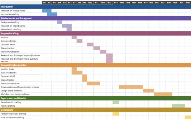
Figure 1.1: Gantt diagram that describes the schedule of this project, where W stands for week.

.

At Figure 1.1 the schedule of this project is visualized, where W stands for week.

At first, it starts with research of various state-of-art topics that finally lead to the topic presented. Various architectures are developed and tested to proof correctness. After tests are performed, and with an acceptable degree of assurance on correctness, these are finally drafted in this document. Encapsulation and model generalization is the step in which an interface is built. The model can process various sizes of matrices, input vectors, and time-steps.

(16)

Chapter 2 Background

This chapter start with a classical computing background, in which the readers first finds an introduction to probability theory. Probability theory is deeply related to both QC and NLP.

Persevering on classical concepts, this chapters devotes a section to introduce NLP:

it gives insights on encoders-decoders and RNN. It does not dive deep into to much details, but it is neither leaving apart important concepts that are needed to understand this work.

The second section of this chapter has the goal to introduce QC. This second part, start with Linear Algebra, that even though it can be consider a classical theory background, the reader will notice that the concepts handed-down are exclusively used though-out this work for QC. Thereafter, the QA paradigm used is explained profoundly since this is the core of the work.

2.1 Classical Computing Background

The nucleus of this chapter is NLP, however in order to understand the discussed models, this work provides to the reader important concepts that are intrinsically present in NLP, and moreover, are somehow important to understand how QC is applied in the following chapters. These important concepts are the ones mentioned in the probability theory part.

With the basic mathematics concepts in mind, the work grasps the language models that it promised to talk about. It discusses Encoders-Decoders,RNN and the sampling problem itself.

(17)

2.1.1 Probability Theory

A very frequent concept in probability theory are random variables, which can describe variables whose values are unknown ¹ [Goodfellow et al., 2016]. Their definition is as follows [Stroock, 2010]:

Definition 1. Let ⌦be a sample space, F be an event space, and P ra probability function that assigns a probability to each event in F. Then a random variable is a function:

X : (⌦,F, P r)!w. Where w can be continuous, discrete, or a non-numeric value.

Random Variables are going to be denoted throughout this work with uppercase letters, and their respective outcomes in lowercase letters. The di↵erent values that these can take are described by probability distributions [Goodfellow et al., 2016]. A technical way to describe distributions is given in Definition 2 [Stroock, 2010].

Definition 2. Let x2⌦, then a probability distribution is a function f :x!P r(X =x).

Probabilities distribution are an introduction to understand likelihoods, which is a tool that helps to quantify and compare how a model distribution is against the true distribution. Likelihoods are discussed in the next section, however a definition to give the reader an idea of this concept is presented as follows:

Definition 3. Let ⌦X,⇥ be the sample space of some random variable X, and some parameters of a model respectively. Then the likelihood is the product of the probabilities that the model with parameters ⇥ assigns to each event of the sample space⌦X (See Equation 2.1).

P r(X;⇥) = Y

x2⌦X

p(X =x;⇥). (2.1)

These concepts are useful when modeling a language since it is required to search probabilities to determine a language sequence, and moreover, it gives an idea on how to test these models. Withal, it must be noticed that the models used are dependent of various variables, and this is why there is a need for additional concepts so a functional model can be built. One of these concepts are Marginal Probabilities.

Marginal probabilities are, redundantly speaking, probabilities for a subset of variables. More formally, these attend to the following definition [Goodfellow et al., 2016]:

Definition 4. The probability that some event on a random variable X occurs is given by the sum of all joint probabilities in which this event happens (see Equation 2.2).

8x2⌦X, P r(X =x) = X

y12⌦_Y₁

· · · X

yn2⌦_Yn

P r(X =x, Y1 =y1,· · · , Yn=yn). (2.2)

1On its counterpart, an algebraic variable can be calculated. E.g x+ 1 = 2 assigns an specific value of 1 tox.

(18)

Joint probabilities are not only useful for marginal probabilities, but also they help us calculating conditional probabilities. These help to determine the probability of some event B happen given that some other event A already had happened. Formally, it can be defined as [Goodfellow et al., 2016]:

Definition 5. Let X, Y be random variables and x,y some state from their respective sample states. Then the conditional probability that Y=y given X=x is denoted as Pr(Y=y | X=x) and it is given by Equation 2.3. In this equation Pr(Y=y, X=x) represents a joint probability.

P r(Y =y|X =x) = P r(Y =y, X =x)

P r(X =x) . (2.3)

If you take Equation 2.3 and multiply each side by P r(X = x) you are left with what is known as thechain rule which can be further expanded as in Equation 2.4, where 8i 1in , xi is the outcome of some random variable Xi.

P r(x1, x2,· · · , xn) =P r(x1) Yn i=2

P r(xi|x1,· · · , xi 1). (2.4)

2.1.2 Natural Language Processing

This research deals with the task of generating a sentence given as input another sentence.

The first sentence in mention is called source sequence, and the second target sequence due to their nature. Moreover, |S| indicated the length of the sentence, Si indicated in 1-indexed notation word i, S_i^j is the sub-string that comprises all words from Si to Sj

(including both start and end). Therefore, S₁^|^S^| =S, and S =S1S2· · ·S_|S|.

Each token of the sequences can be represented in various ways, however in this research we are going to deal with one-hot encoding vectors. This is a vector whose elements are either 0 or 1, however only element equals 1. Each index maps to a word.

Therefore depending which element of a one-hot encoding vector equals 1, it can be known what word it refers to.

Producing a target sequence from a source sequence is actually a conditional probability, were the task is to calculate the probability of some target sequence given a source sequence.

In Natural Language processing an Encoder-Decoder is used to process a source sequence and to produce a target sequence. Their architecture can be seen at figure 2.1 and can be summarized as follows:

1. Encoder: This part is an RNN that receives at each timestep a token, finds its representation (i.e one-hot vector encoding), and process it. At the end of the encoder section it will output the input of the decoder part.

2. Decoder: The decoder process the output of the encoder and outputs a token for each timestep. In this work, the only input each timestep receives is the output of

(19)

the previous timestep. This is just to reduce the number of variables, however is easy to add this input to overall proposal of this research.

Figure 2.1: Encoder-Decoder architecture in which lookup^(f) designates a word representation for the word input fi (similarly is done with lookup^(e)), and the soft-max refers to the soft-max function, which outputs a probability distribution over a set of vocabulary words [Neubig, 2017].

.

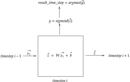
Going deeper, a RNN is shown in Figure 2.2. In this figure, each time step receives an inputxtof the previous timestep, except for the first time-step which receivesx0. Also, it can be seen that each time-step outputs a vector, i.e. ht. In Figure 2.3 a more specific view can be seen. Even though, there are various things that can change between models, these ideas do not vary greatly.

In the last mentioned Figure, W is a weight matrix which is multiplied by the input (i.e !xi) of each time-step, and then, summed towards a bias (i.e !

b ). W!xi +b is known as an affine function.

The result, let it be !z, is then used as input for an activation function. When this function is applied, we get y which is a vector that may represent the likelihood of seeing token y_i. Therefore the result of this time-step is the word mapped by the index whose likelihood is the biggest. Finally, result time step can be transformed again into a one-hot encoding vector and become the input of the next time-step.

The task of decoding and finding the set of k best target sequences is known as sampling and it is a NP problem. Let the target sequence beS, then the scope is to find suchSthat the maximal conditional probability for all marginal probabilities is maximized (see Equation 2.5).

S =argmax(

Y|S|

t=1

P r(St|S₁^t ¹)). (2.5)

The standard sampling algorithmsare 3 [Ippolito et al., 2019]:

(20)

Figure 2.2: A simplified view of the structure of the RNN architecture.

.

Figure 2.3: Inner view of each time-step of an RNN.

.

• Random Sampling chooses the a random word in each time-step.

• Greedy 1-Best Searchchooses greedily in each time step the word that, when added to the target sequence, gives the highest probability.

• Beam Sampling (BS) is very similar to Greedy 1-Best Search, with the only di↵erence it searches for k target sequences.

The discussed sampling algorithms show a lack of method to obtain the best possible answer, since neither randomly or greedily ensure an optimal result.

(21)

2.2 Quantum Computing

This second section deals with mathematics behind the sub-atomic world that are used to make functional quantum computer algorithms. The now in mention section starts in bottom-up manor explaining the mathematics concepts, and how this are used to concretely explain quantum mechanics concepts. Built upon this concepts, is where a quantum paradigm called Adiabatic Quantum Computing (AQC) is found, in which at the same time comprises QA. The notions of this paradigm are explained in this last part.

2.2.1 Linear Algebra and Quantum Mechanics

To understand the properties Quantum Mechanics have to o↵er the readers needs to keep in mind that quantum laws are possible because it operates within a Hilbert Space [Laforest, 2015].

Definition 6. A Hilbert Space is a vector space with a well defined inner-product [Laforest, 2015].

Definition 7. A vector space is a set of vectors with same dimension that meet the following properties [Laforest, 2015]:

• The set is closed under addition and multiplication, if 2 vectors are added and/or multiplied, then the result is also in this set.

• Let #»

x , #»

w and #»

v be vectors of a vector space V, and c, d be scalars. Then these scalars and vectors meet the following properties:

– Commutativity: #»

x +#»

w = #»

w+#»

x. – Associativity: (#»

x + #»

w) + #»

v = #»

w+ (#»

x +#»

v).

– Distributivity of scalar multiplication: c(#»

x + #»

w) =c#»

x +c#»

w.

– Distributivity of scalar addition: (c+d)#»

x =c#»

x +d#»

x. Definition 8. Let #»

x ,#»

w be vectors with same dimension. Then the inner product of these vectors is denoted by #»

x•#»

w and it equal the sum of every element-wise between these 2 vectors (see Equation 2.6) [Laforest, 2015].

#»x • #»

w =X

j

xjwj. (2.6)

Quantum Mechanics have various dimensions, and whenever 2 quantum systems collapse, new possible quantum states are created. A mathematical way to describe this process is through tensor product that can be generalized to the Kronecker Product [Nannicini, 2017].

(22)

Definition 9. Let A 2 C^mn and B 2 C^pq. The Kronecker Product known as A⌦B is a matrix S 2C^mp⇥nq

S :=A⌦B = 2 64

a₁₁B · · · a_1nB ... . .. ...

am1B · · · amnB 3 75.

Tensor product is used to represent states of various qubits. Qubits are the coun- terparts of classical bits but the di↵erence is that other than being just in state 0 or 1, they can be in both state at the same time and this is called superposition. To denote states, quantum computing literature uses Dirac’s Bra-ket Notation whose definition is as follows.

Definition 10. | i denotes a column vector defined in a complex Euclidean Cⁿ, and h |2 (Cⁿ)^⇤ denotes a row vector and the conjugate transpose of | i.

|0i=

1

0 ,|1i=

0

1 . (2.7)

The basis states of one qubit is in Equation 2.7. However, this can be extended to states of various qubits. For example, if there are 2 qubits, then 4 basis states can exist (i.e. doing tensor product between 2 states of qubits): |00i,|01i,|10i, and |11i. These, just as in Equation 2.7 can be all represented in a ket defined in a complex Euclidean space C⁴. A further generalization can be formally defined.

Definition 11. Let C² be a standard basis defined as in Equation 2.7. Basis states can be obtained of q-qubits by applying tensor product various times to the so far defined standard basis C² and it is denoted as (C²)^⌦q.

The reader might notice that the number of basis states increases exponentially with the number of qubits used. That is why it is convenient to use a notation to express binary string that can later be used to represent basis states [Nannicini, 2017].

Definition 12. Let l be an integer greater than 0, then #»

j refers to a binary string, i.e.

#»j 2 {0,1}^l and the n-th digits of it is denoted by #»

j_n. This system uses the first digit as the most significant one (little-endian convention). More on, when using it within a ket or a bra, the length of this string is of size q, and is denoted by writing |#»

ji_q.

Having this notation, now various properties can be generalized regarding basis states, and properties like entanglement and superposition for one or more qubits.

To describe the state of a system of qubits it is used a linear combination as described in next proposition.

Proposition 1. Let |!i be the state of and q-qubit system, then its state is going to be a linear combination [Leonard Susskind, 2014] of basis states. Generally the state is described as

|!i= X

#»j2{0,1}^q

!^#»_j |#»

jiq,8!^#»_j 2C. (2.8)

(23)

The coefficients that multiply each basis state are known asprobability amplitudes and they take values ranging from 0 to 1, thus !^#»_j!^⇤^#»_j is the probability of measuring the state it is coefficient of [Leonard Susskind, 2014].

Given the generalization (Equation 2.8) of a state,Superpositionandentanglement can be defined.

Definition 13. Given a q-qubit system, and the state of this system denoted by |!i = P#»

j2{0,1}^q!^#»_j |#»

jiq, then this system is in a basis state if and only if 9^#»k : !^#»_k = 1 and 8#»

j 6= #»

k ,!^#»_j = 0. Otherwise the system is in superposition [Nannicini, 2017].

Superposition happens when there are various probabilities of measuring di↵erent basis states deduced from the coefficients !^#»_j.

Tensor Products helps to define what a product state is, and product states helps to define what entanglement is. The formal definition is described next.

Definition 14. A quantum state system ! 2(C²)^⌦q is a product state if it can be written as tensor product of q 1-qubit states. Otherwise it is entangled [Nannicini, 2017].

For example, suppose there is a 2-qubit entangled system, then Equation 2.9 is a product state since it is equal to (^p^|⁰ⁱ₂ +^p^|¹ⁱ₂)⌦(^p^|⁰ⁱ₂ +^p^|¹ⁱ₂) [Nannicini, 2017]. But Equation 2.10 is not [Nannicini, 2017].

|!i= |00i

2 +|01i

2 +|10i

2 + |11i

2 , (2.9)

|!i= |00i

2 +|11i

2 . (2.10)

Figure 2.4: Block Sphere that have 3 basis states represented in x, y and z axis. The dot is representing a particle in superposition and the block sphere helps us giving a position to it [McGeoch, 2014]

.

Basis states are a very abstract definition, but what they are really doing is representing some measurable ². To understand better basis state, an analogy of a measurable

2known in quantum textbooks as observables

(24)

to the atomic world can be done: for some atomic-sized mass, we can easily study its position and velocity, these properties are an analogy of a measurable in the quantum world.

A measurable, is thus a property of some sub-atomic-sized being (e.g photon, electron, quark) like spinning orientation [Leonard Susskind, 2014]. Heisenberg’s Uncertainity prin- ciple tells something regarding measurables [Leonard Susskind, 2014]: the most is known about a measurable, the less is known about some other. This is the reason why the next proposition comes out to be trivially true.

Proposition 2. Recall Equation 2.8. The norm denoted by || |!i|| is a unit vector (i.e.

equals 1) and is equal to p

h!| |!i.

Having normalized states for qubits are useful cause they can use the Block Sphere to represent the position of a qubit (See Figure 2.4). Even Though, other basis rather than |0i and |1iare defined, 2 things on the Block Sphere can be observed:

1. h1| |0i=h0| |1i= 0 which means they are parallel.

2. h1| |xi=h0| |yi= 1, that means they are orthogonal.

It is out of the scope to show how these basis are defined but the reader might have notice it is not difficult to do some calculation over the standard basis|0iand|1ito obtain other basis. Instead, this basis are now defined:

Definition 15. Let|+irepresent the positive part ofxaxis of the basis state seen in Figure 2.4 and | i the negative part of the just mentioned axis. Then these are orthogonal to kets |0i and |1i and they are defined as [Asfaw, 2020]:

|+i= |0i+|1i

p2 ,| i= |0i |1i

p2 . (2.11)

Definition 16. Let|ii represent the positive part of y axis of the basis state seen in Figure 2.4 and | ii the negative part of the just mentioned axis. Then these are orthogonal to kets |0i and |1i and they are defined as [Leonard Susskind, 2014]:

|ii= |0ip+i|1i

2 ,| ii= |0ipi|1i

2 . (2.12)

Recall that previously it is said that measuring the outcome is measuring some property of a particle. It can be imagined as having a device that reads according to the basis defined in Equation 2.7 but other basis may be used. Quantum computing always do measurements under the basis states |0i and |1i and even though it can conserve uncertainty under other basis after doing measurements under classical basis states, the real reason to define other basis is because in this manner, qubits can be moved in various ways, and thus achieving a more variety of operations, that can be visualized in the Block Sphere.

(25)

2.2.2 Quantum Annealing and Adiabatic Quantum Computing

QA shares aspects with AQC, which at the same time is a type of a Universal Quantum Computer (UQC). The di↵erence between a UQC and an QA is that the first one is meant to be used with any type of problem, while AQC is meant to be used only to solve optimization problems [DWave, 2018]. While UQC tries to control in every aspect the qubits, AQC treats particles as a whole, and tries to give them shape as if they were some sort of mass. This di↵erence makes a whole easier to scale with accuracy QA and that is why it turned-out to be the leading paradigm for QC. In the following paragraphs it is explained the shared aspects of QA and AQC.

Figure 2.5: The various types of QC and how UQC relates to QA [DWave, 2018].

.

AQC is inspired on quantum dynamical systems that evolve through time [McGeoch, 2014] and is a system that consist on forces that can be rather external or qubit-produced.

AQC evolves qubits over time, as if they were particles, by making use of forces. These are represented with a time-varying Hamiltonian Ht matrix of sizenxn and every observable state has an associated energy that depends on Ht [McGeoch, 2014].

The set of all possible energies is calledenergy spectrumand it has two main states:

1) the lowest possible energy state, called ground state and 2) a state that is not ground state is called excited state [McGeoch, 2014].

AQC algorithmms have the following components [McGeoch, 2014]:

• An initial Hamiltonian (HI) in which it appends every possible observable state (i.e.

qubits are in superposition).

• The final Hamiltonian (HF) encodes the minimum eigenvalue and an eigenstate of the register of qubits. This is an optimal solution of given objective function and applies energies according to the model proposed for an specific problem. Qubits are altered through time.

• An adiabatic evolution path (s(t)), that decreases from 1 to 0.

(26)

The idea is to create a gradual transition from an initial Hamiltonian to a final one according to Equation 2.13 and according to the adiabatic theorem it will almost for sure return an optimal solution [McGeoch, 2014].

H(t) =s(t)HI + (1 s(t))HF. (2.13) A type of AQC is QA which is a technique developed for combinatorial optimization problems and for classic computers, but as the name suggest it is meant to be used with quantum computers. D-Wave quantum computers are quantum annealers. An explanation of how this works follows.

Each qubit have a circulating current and is associated to a magnetic field see Figure 2.6. It is important to remark that because these are quantum objects, they can spin in more than 1 direction.

Figure 2.6: Clockwise current is associated to a state |0i and counter clockwise is associated to |1i and the arrows represent a magnetic field [DWave, 2018].

.

Generally, the process of quantum annealing can be summarized in Figure 2.7. This process describes 3 main stages of QA: at first all qubits are in superposition and this is the a low energy state, then a programmable quantity of force is applied in the respective associated magnetic field within each qubit (called bias), to finally get a lower energy for certain states, and thus a higher probability of measuring it.

Figure 2.7: Set of images evolving through time, and a) representing time 0. These images represent main stages of quantum annealing and how applying a magnetic field results in getting a higher probability for a 1 [DWave, 2018].

.

A special type of relation between qubits can be created by using couplers. This relation between qubits known as entanglement, can be programmed with a parameter called coupling strength.

(27)

When trying to solve a problem using quantum annealing, the first step is to state the problem as in Equation 2.14 which is the same as Equation 2.13 but more specific [DWave, 2018]. _x,z are Pauli matrices,h_i are the biases associated within each qubit i, andJ_i,j is the coupling strength between each pair of qubit (i, j) [DWave, 2018].

H = A(s) 2 (X

i (i)

x ) + B(s) 2 (X

i

hi (i)

z +X

i>j

Ji,j (i) z (j)

z ). (2.14)

Pauli matrices areQuantum Gates, and these are used to transform states of qubits, which in other words, means they move the qubits along the block-sphere. The formal definitions are as follows:

Definition 17. Let M denote a quantum gate and M^⇤ the complex conjugate of M. Then if M^⇤M =M M^⇤ =I, M is unitary [Nannicini, 2017].

The basic quantum gates are given by Pauli matrices which are:

I =

1 0

0 1 , X =

0 1 1 0 , Y =

0 i

i 0 , Z =

1 0

0 1 .

Even though the reader now knows what the Pauli Matrices are, an explanation of Equation 2.14 is still in debt. The first term of Equation 2.14 is trivial since it is only the qubits in superposition, therefore a brief explanation on how can to get the second term follows. To get the second term of Equation 2.14, it is defined an objective function using an Ising model or a Quadratic Unconstrained Binary Optimization (QUBO)³ model.

First, the Ising model is defined as Equation 2.15 and it can easily be seen that this is the second term of Equation 2.14. However, it can also express an objective function as a QUBO which is a way to define a problem within an upper triangular matrix. Then, the QUBO matrix, denotated as Q, can express the objective function as in Equation 2.16.

I = XN

i

hisi+ XN

i=1

XN j=i+1

Ji,jsisj, (2.15)

f(x) =X

i

Qi,ixi+X

i<j

Qi,jxixj. (2.16)

The only di↵erence between QUBO and ISING is that in the QUBO model random binary variables take values of 0 or 1, while in the ISING model, variables take values of -1 or 1. This work uses the ISING model because its easier to find global optimums in it.

3It is unconstrained because there are no constraints other than the ones defined in the formulation of the objective function.

(28)

Another way of seeing Equation 2.16 is that the diagonal terms are the linear coefficients, and the upper diagonal elements are the coefficient of the quadratic terms [DWave, 2018].

Objective functions can also be represented with graphs. Suppose there are 2 qubits a and b, and an objective functionf(a, b) = 5a+ 7ab 3ab, the a graphical representation is seen in Figure 2.8.

Figure 2.8: These image represents an objective function in which 5 and -3 are the biases of a and b respectively, and have a coupling strength of 7 [DWave, 2018].

.

The Dwave architecture and qubit disposal is aChimera Graphsuch as the one seen on Figure 2.9. Chimera Graphs are made upon various k4,4 sub-graphs, and this is very important to consider and thus, it also explains why it can express objective functions as QUBOs.

Figure 2.9: Chimera graph. Circles represent qubits and edges are the couplings between these [DWave, 2018].

.

To program the Dwave quantum computer, we have to install the SDK: dwave- ocean-sdk through pip install. Afterwards, a problem can be formulated and sent to the quantum computer as in Algorithm 1.

The example displayed at Algorithm 1 minimizesf(q1, q2) = 2q1 2q2+ 3q1q2, where q1, q2 2{ 1,1}. Therefore the answer should be q1 = 1 andq2 = 1 since this evaluates f(q1, q2) = 7, and every other possible configuration gives a greater value for f.

In line 1 we created an object that has various methods including the one from lines 2 to 4.

When the SDK is installed it creates a file called dwave.conf which contains the name of quantum computer, the architecture of the Quantum Processor Unit (QPU) among other settings. This settings are loaded in line 5. Since qpu already contains how the qubits are arranged the functionEmbeddingComposite(qpu)does the mapping to physical qubits.

(29)

When no embedding is possible because some variable has more than 4 connections⁴ it will try to add extra variables known asancillas. Ancillas represent one logical variables even though multiple qubits represent it. The chain strength of line 7 is the coupling strength by which these ancillas are connected⁵

Finally, line 8 gets the result with the lowest energy since we had performed 100 reads, and we can map the names of the qubits (i.e q1 and q2) to the result.

2.3 Final Remarks

In the next section it is presented the related works in which all these concepts are mentioned or are somehow present. This chapter is worth reading to grasp in detail the evolution of the upcoming works and to understand how the proposal of this work flows.

Algorithm 1:Example of how to program a quantum computer.

// Suppose we want to minimize f(q1, q2) = 2q1 2q2+ 3q1q2

// Create a dictionary to save coefficients

1 bqm dimod.BinaryQuadraticModel.empty(dimod.SPIN);

// add linear coefficients

2 bqm.add variable(‘q1’, 2);

3 bqm.add variable(‘q2’, -2);

// add quadratic coefficients

4 bqm.add interaction(‘q1’, ‘q2’, 3)

// Load configuration from file dwave.conf

5 qpu DWaveSampler(solver=‘qpu’: True);

// Map logic variables to physical qubits

6 sampler EmbeddingComposite(qpu);

// Sample the quantum computer

7 result sampler.sample(bqm, num read=100, chain strength=3) // Get answer with the lowest energy

8 result result.first.sample

9 q1 result[‘q1’];

10 q2 result[‘q2’];

4Recall the QPU-architecture is ak4,4 graph.

5The chain strength is always positive. Additionally, is always recommended that its value is the biggest absolute value that any coupler can take.

(30)

Chapter 3

Related Works

The goals of this chapter are two:

1. Give a fast introduction of current-state-of-art samplers for Seq2Seq models such that the importance of developing a new sampling method is understood. We show that this research is relevant.

2. Show that this research is novel in various aspects, and have the potential to highly contribute the research community.

3.1 Sampling Methods for Decoders

As far as we know, there are no research studies on how QA can be applied to the sampling task of Seq2Seq models. Some of these works have focused on learning word embeddings [Zeng and Coecke, 2016, Srivastava et al., 2020]. The word representation using quantum mechanics is greatly encouraged by [Li et al., 2018], since the authors proof that a quadratic speedup can be achieved with quantum properties, and moreover additional properties can be naturally expressed with these quantum properties.

Recently, Recurrent Neuronal Networks have been proposed either in a theoretic way, hybrid, or with another quantum paradigm (i.e gate-based). A gate-based approach [Bausch, 2020] develops much slower compared to quantum annealing. Further on, this was only tested within a simulated context on a classical computer.

Insights of how quantum computing can substantially decrease running time of NLP decoders and a theory to build a quantum-based decoder have been also proposed [Bausch et al., 2019].

Our proposal is greatly di↵erentiated because it was tested on a real quantum en- vironment and we are using QA to solve a very hard problem that has an exponential complexity.

A first sampler was proposed by [Sutskever et al., 2014] in which the heuristics,

(31)

according to the author, are justified by the simplicity of the algorithm. However, later, various authors realized that for real world application, this algorithm is not enough.

There are various work that intend to mitigate the samplers ability to output at least an answer with some degree of sense. It is very common that this answers output something generic such as: I don’t know. One of the works that attempted to do this is [Li and Jurafsky, 2016] which usesMutual Information (MI) to increase the score of the generated sequence. However, it was not space efficient because still with a high beam size it did not achieve encouraging results. Moreover, most of the sequences were very similar.

Instead, our proposal will not go through a search-space in a sequential manner because it uses the mathematical background of QA to compute all time-steps at once.

Other attempts to increase the e↵ectiveness of standard algorithms (i.e. beam sampling, random sampling, and greedy 1-best search) are seen in [Fan et al., 2018], [Tam, 2020] and [Vijayakumar et al., 2016]. However, they increase space complexity, increase the algorithm complexity, and they reduce the search space. Additionally, [Fan et al., 2018]

shows how current heuristics will fail for long sequences and arguably, the best answers have been pruned by the authors of all the aforementioned works. Thus, we realize that we are dealing with an NP problem, and it cannot be solved by the classical-mechanics-based approach.

3.2 Final Remarks

QC is a very encouraging technology that has the potential to increase e↵ectiveness and efficiency of current state-of-art methods. However, there are no works regarding on how QA can be applied to the sampling task, and furthermore there are no empirical studies done in QC for NLP. These facts gives our proposal the attributes of relevant and novel.

Currently classical-based methods are not efficient in terms of space and time complexity. Additionally, they struggle to find good answers. The di↵erence between these methods and ours is that the first decode a time-step in a blindly manner. However, with the properties of the quantum world and the mathematical basis of QA we can compute all time-steps at once considering an answer that maximizes the score of all the time-steps.

(32)

Chapter 4

The Proposed Method

This chapter will propose a new method for sampling Seq2Seq models of NLP by first giving an initial intuition. Then, we start working on the components to build a sampler for RNN. Later, it describes how these can actually be used to build this sampler.

The overall complexity time of the proposal is given byO(n³⇤T), where n is the size of the input vector, and T is the number of time-steps. This complexity is given by the steps needed in order to build a dictionary that represents the force fields and coupling values.

This dictionary is built with a classical computer and then is sent to the quantum computer through an Dwave API.

4.1 Intuition

Neural networks will encounter the following expression:

!y =argmax(sigmoid(W!x +!

b )), (4.1)

(a) Graph of thesigmoid function.

.

(b) Graph of thetanhfunction.

. were!y ,!x ,!

b are column vectors which represent the output, input, biases, and W is a weight matrix that is trained so it can correctly output y.

(33)

In our context, x is a vector with binary random variables. However we are going to work with an ISING model. Therefore zeros are represented by -1.

In every time-step y is computed. Therefore, a vector of random binary variables, where the index with maximum likelihood is represented by a 1, otherwise yi = 1.

Even though most models nowadays contain more than just one equation like Equa- tion 4.1, it must be noticed that discovering how to build this basic block will lead us to a solution.

More over, the reader might had noticed that there are also tanhs in these other models. But, at the endtanhs and sigmoidhave the same scope in terms of output. The only di↵erence between them, is that the gradient of tanhs can help the model in the vanishing gradient problem at training time.

In figures 4.1a and 4.1b the reader can see the sigmoid and the tahn function respectively. Moreover, it can be seen that in both of them, that when the input variable has positive value then the output variables tends to be 1, otherwise 0. In the case of the tahn function, -1 instead of a 0. Which in both cases represent logical ones or zeros respectively.

The just mentioned fact is a kickstart to start analyzing these random binary variables in such way these can be represented in a quantum computer. Giving a concrete and small examples each of these vectors and matrix can therefore be:

W =

w11 w12

w21 w22 =

 1 2

3 4 , x=⇥ x1 x2

⇤ =⇥ 2 3⇤

, b=⇥ b1 b2

⇤ =

 5

1 , (4.2) y=

y₁

y2 =argmax(sigmoid(W x+b)). (4.3) At first, this work will work with just sums to start with the very basic. So multi- plying W and x implies

W x=W x=

( 1)⇥2 + ( 2)⇥3 3⇥2 + 4⇥3 =

 8

18 . (4.4)

At this point there is only one step missing which is that it must sum b. If the sum and the sigmoid function is applied, this leads to

y=sigmoid(W x+b) = sigmoid(

 8 18 +

 5

1 ) =sigmoid(

 14 19 ) =

0

1 (4.5)

From this, two theorems can be stated:

Theorem 1. If w_ij and x_k are being multiplied then:

(34)

• if wij and x have di↵erent signs then y is more likely to be negative.

• Otherwise y is more likely to be positive.

Theorem 2. If b is positive then y is more likely to be positive, otherwise negative.

This being said, now it proceeds to state how this can be related to QA. It is the moment that the reader recalls the ISING function:

f(X) = Xn

i

hi⇤ri + Xn

i

Xn j=i+1

Jijri⇤rj. (4.6)

In Equation 4.6 the reader shall recall that the lineal coefficients (i.e. hi) represent a force field being applied to a qubit that will determine, at the end of the annealing, the spin. At the same time, depending of its direction,the spin represents a -1 or a 1.

On the other hand, the quadratic coefficient (i.e. Jij) will determine the coupling strength, this means the force by which 2 qubits are entangled.

The reader shall also recall that this function is being minimized and this gives us the following rules:

Theorem 3. Let ri be a binary variable whose result 2 { 1,1}, and hi is its respective force field. Then:

• If ri is positive then in order to minimize the ISING function, hi must be less than 0.

• If ri is negative, then hi must be set to a value greater than 0.

• If hi is exactly 0 then it can be said that the quantum system has equal probabilities for outputs -1 or 1 and it depends on coupling values (i.e. neighbors of ri) which value it takes.

Theorem 4. Let ri, rj be a binary variables whose result 2 { 1,1}, and Jij is their respective coupling value. Then:

• Without loss of generality, if ri is negative and rj is positive (i.e. have di↵erent signs, then the coupling value should be positive in order to minimize the ISING model.

• If both binary variables have equal signs, then the coupling value should be negative.

• Finally, if the coupling value is 0, then ri and rj cannot imply signs.

Assume we want to compute y = sigmoid(a+b), where a and b are real numbers and our aim is to determine whether y is activated or not. Let|a|<|b|, a >0 and b <0.

Therefore, a+b <0 andyshould not activate. Additionally, every constant and the result

(35)

have their own qubit assigned: qa, qb and qy respectively. Each assigned qubit represents the sign.

Therefore, h_a, h_b can be set equal to a and b respectively, and h_y to 0 since we do not known its sign. Moreover, we can also set Jay = |a| and Jby = |b| since qa and qb both want qy to have the same sign as theirs. However, since |a|<|b|, qy must obey qb

sign so that the overall ISING is minimized.

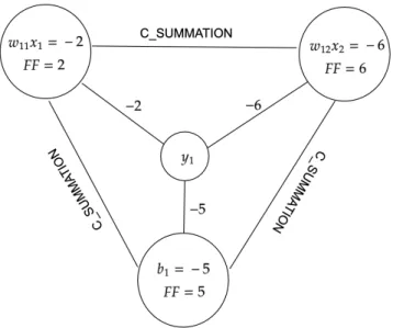
This idea can therefore be applied to represent summation architecture which in- cludes intrinsically an activation function(see Figure 4.2), and that works with an arbitrary number of operands.

Figure 4.2: Architecture 0: represents the sum of 3 variables in order to get the sigmoid value of a random binary variable yi. FF stands for ”force field”.

.

4.2 Bottom-up approach to Build a Quantum Sampler

The purpose of this section is to explain how a sampler for RNN can be built using quantum computer in a bottom-up manner. First, it will explain how the sign of a multiplication can be extracted. Second it will show how various rows can be multiplied by various columns, and output a sigmoid function based on these operations. Third it will show how to penalize output qubits so only one element of the output vector is selected. Last it will show how all these parts can be connected to build an RNN.

4.2.1 Extracting the sign of a Multiplication

A way to get the sign of a multiplication is seek. The intuition for the next architecture is to be thought in a way that signs are represented as qubits, i.e:

(36)

• If the sign is negative, a positive force field has to be applied to a qubit so it can be forced to have a value of -1.

• Otherwise apply negative force field.

Let’s denote these input qubits as I1 and I2, and the output qubit as qo. Then, the above intuition leads to the need of building an XNOR gate since this gate will, eventually, allow qo to be 1 if I1 and I2 are equal, otherwise it should be equal to -1.

Even though, using a NOR gate is also valid (since it is just a matter of playing with an inversed output), an XNOR gate can be constructed more efficiently.

According to [DWave, 2018], every boolean circuit can be built on a quantum computer. Therefore, the rules to entangle and to set the force field of input and output qubits of an XNOR quantum gate should be seek.

Figure 4.3: Boolean circuit of logic NAND.

.

Figure 4.4: Architecture 1: Architecture that represents a logical NAND. At the left-hand side the reader can see how qubits are displayed following the letter notation of 4.3. At the right-hand side the force fields in each circle, and the coupling values near the edges is being displayed.

.

An XNOR gate can be built with 3 NAND gates according to Figure 4.3. A NAND gate, denoted as Architecture 1, can be built without ancillas as shown in Figure 4.4.

The explanation of this architecture and considerations are given next:

• A and B are input qubits, and C is the output qubit of a relative NAND gate.

• Input qubits need to have a larger absolute-valued force field applied than the output qubit. This is why, intuitively 2 is chosen as the force field of input qubits and

(37)

-1 for the output qubit. This is because input qubits seek to ”influence” the output qubit.

• The reason why input qubits are being divided by their absolute value is because those qubits are only representing signs (at least by the moment).

• The couplers are set to 1 because this is how the energy function can be minimized when di↵erent signs are received.

• The output qubit receives a force field of -1 because if the output qubit is set to 0, then the energy function is equal when both signs are the same, so in order to get an energy less than 0 when both sign are negative, the output qubit is set to -1.

The proof of correctness of quantum NAND gates is straightforward:

Proof. Let qa, qb, qr be the qubits that represent A, B, and the result qubits respectively.

Following Fig. 4.4, then ISIN G_nand = 2q_a 2q_b q_r +q_aq_r +q_bq_r. The following scenarios are given:

• qa and qb have a +1 spin. ThenISIN Gnand= 4 +qr and its ground state is when qr <0.

• qa and qb have a 1 spin. ThenISIN Gnand = 4 qr and its ground state is when qr >0.

• qaand qb have di↵erent spins. ThenISIN Gnand= qrand its ground state is when q_r >0.

Once having a defined quantum NAND gate, a XNOR gate can be built. This works very straightforward: just entangle output qubits of the leftmost NANDs (Figure 4.3) as if these were input qubits (i.e. setting coupler values of these two with the final output to 1), and initialize with proper force fields A, B and their negations according to the signs of the input.

4.2.2 Building Matrix Multiplication

What follows next is to represent a row ofW multiplied by a column ofX. However before going through these rules is important to take into consideration the following facts:

• The absolute value of the force fields of input qubits in XNOR gates have to dominate output qubits.

• Since the multiplication is made of a real number (W) and ones (xi), then it have to only take care of which number does W has.

(38)

Figure 4.5: Intuition of Architecture 2. This image represents a multiplication between 2 numbers (in which one of them is either 0 or 1), and an addition of a bias to this multiplication.

.

• According to the sum representation (i.e. Architecture 0), the coupling values between the qubits that represent the multiplication between X and W have to be proportionally to the same, and the same applies to the elements of the vector of biases.

According to various test a workingArchitecture 2can be built to represent matrix multiplication with the following rules:

1. For each multiplication:

(a) Apply XNOR gates to the operand of the current multiplication according to Architecture 1 to build this gate.

(b) Since it has to proportionally imply the energies in the objective function, and input qubits have to be greater, the input qubits are multiplied by twice the absolute value of the respective W value.

(c) Each output qubit in the NAND gates of the XNOR gate is multiplied by the absolute value of the respective W value.

(39)

(d) Entangle the first two NAND gates by setting a coupling value of C XNOR.

This will force this qubits to have an equal state and the reason of doing so is because of the nature of XNOR gate.

2. Following Architecture 0, entangleyi with proportional coupling values, andbi with the output qubit of the various XNOR gate.

3. The target variable,yi, is in perfect superposition state.

Without loss of generality, an intuition of this architecture can be seen in Figure 4.5 since it display the major components. When more multiplications are added, XNOR gates are built following the rules comprised in point one, and entangle the output qubit of the XNOR gates to y according to rule 2.

4.2.3 Choosing One Value

Once matrix multiplication is done, it will give all the elements of vector Y. There can be various ones, but the overall approach to RNNs require to only have one, and the strongest should dominate.

Intuitively, we can think to entangle all elements of y with a coupler value greater than 0.

In [Nguyen et al., 2014] a method for feature selection is developed. However the useful part of this [Nguyen et al., 2014], is the approach taken to choosek features, since the method proposed in our work seeks to select k = 1 elements of y. This approach states that the following equation is useful:

P =↵

|y|

X

i=1

(yi k)². (4.7)

In Equation 4.7 P can be described as a penalization function and must be added to the overall QUBO model.

In 4.7 ↵ must be chosen. The author states that given a sufficiently large alpha then the quadratic function can guarantee that solutions with a di↵erent number k = 1 ones will be no longer minima. From this equation it can be inferred that the approach followed so far can be still used. This can also be validated with DWave’s function dimod.generators.combinations(), and by setting the parameterstrength=↵.

By runningdimod.generators.combinations() it is seen that the coupling values are set twice the strength, and that every yi must be entangled to the other |Y| 1 elements. Moreover, each yi is set to |↵|, but later test will determine if force fields on each y_i should be applied since these can a↵ect the architectures developed so far.

(40)

4.3 Quantum Sampler

Finally, each time step must be connected.

There are various ways to connect time-steps. In our test the approach displayed at Figure 4.6 proved to achieve e↵ective results.

The idea is to apply the affine function and the sigmoid function once, this result is kept in a set of random binary variables (zi), and an additional copy is added. The copy z copyi is formed by creating the same couplers that zi has with the overall structure (i.e the rectangle with rounded corners of Figure 4.6).

Algorithm 2:Building a Timestep.

Result: ansi,zi

// W: weight matrix.

// x: input of the previous timestep.

// x_names: names of the variables.

// b: bias.

// bqm: current binary quadratic model.

// t: current timestep.

// define a prefix to name qubits/variables of this timestep.

1 prefix to string(t)

2 w names get names(w, prefix + ‘w’);

// Perform multiplication and return operands for summation.

3 operands matrix vector multiplication(bqm,w, w names, x, x names);

// Declare return values.

4 x next [];

5 x next copy [];

// Summation and sigmoid function

6 for i 0 to operands.size() do

// add corresponding bias to operands

7 operands[i][prefix + ‘b’ + i] b[i];

// make 2 copies of the result of this timestep

8 quantum sigmoid sum(bqm, operands[i], prefix+‘target’+i);

9 quantum sigmoid sum(bqm, operands[i], prefix+‘target c’+i);

10 x next.add(prefix+‘target’+i);

11 x next copy.add(prefix+‘target c’+i);

12 end

// Apply argmax only to only one of the copies

13 bqm.update(dimod.generators.combinations(x next, 1,strength=↵));

14 returnx next, x next copy;

The scope of making a copy is to be able to directly connect time-steps without applying theargmax func