A THESIS SUBMITTED IN PARTIAL FULFILMENT OF THE REQUIREMENTS FOR THE DEGREE OF

(1)

ANALOG FABRICATION OF PID

CONTROLLER

A THESIS SUBMITTED IN PARTIAL FULFILMENT OF THE

REQUIREMENTS FOR THE DEGREE OF

Bachelor of Technology

in Electrical Engineering

By

Tapan Kumar Swain

Vaibhav Baid

Under supervision of

Prof. Sandip Ghosh

Department of Electrical Engineering

National Institute of Technology, Rourkela

(2)

CERTIFICATE

This is to certify that the project entitled, “Analog fabrication of PID Controller”

submitted by Tapan Kumar Swain and Vaibhav Baid is an authentic work carried out

by them under my supervision and guidance for the partial fulfillment of the requirements

for the award of End semester thesis Submission in Electrical Engineering at National

Institute of Technology, Rourkela (Deemed University).

Prof. Sandip Ghosh

Rourkela Dept. of Electrical Engineering, National Institute of Technology,

(3)

ABSTRACT

The PID controller has been used and dominated the process control industries for

a long time as it provides the control action in terms of compensation based on

present error input(proportional control), on past error(integral control) and on

future error if recorded by earlier experience or some means(derivative control).

The PID controllers have excellent property of making the system response faster

and at the same time reduce the steady state error to zero or at least to a very small

tolerance limit. The work below starts with study of individual components of the

controller and their responses in a certain environment for different test signals

(say a step or sine wave input).The problem is to design a PID controller using

appropriate analog circuit as well as understand and utilize the advantages of all

the three terms. The below work is for the study of an analog PID controller using

operational amplifiers and fabricate the controller on hardware after testing the

(4)

ACKNOWLEDGEMENT

We express our gratitude and sincere thanks to our supervisor Prof. Sandip Ghosh,

Professor Department of Electrical Engineering for his constant motivation and

support during the course of our thesis. We truly appreciate and value his esteemed

guidance and encouragement from the beginning of our thesis. We are indebted to

him for having helped me shape the problem and providing insights towards the

solution.

We, Tapan Kumar Swain and Vaibhav Baid, are thankful to each other for

co-operating and encouraging and being alongside for the literature review and

background study, the hardware implementation, experiments and the whole thesis

in the same project work.

We extend our gratitude to the researchers and scholars whose hours of toil have

produced the papers and thesis that we have utilized in our project.

(5)

LIST OF TABLES



TABLE 1:-

Transfer function of various controllers using Op Amps 17



TABLE 2:-

Effects of increasing a parameter independently 21



TABLE 3:-Datasheet of LM741

23



TABLE 4:-

Components used in fabricating PID controller 31

LIST OF FIGURES



FIGURE 01:-

Block diagram of a PID controller 14



FIGURE 02:-An inverter circuit

16



FIGURE 03:-C

ircuit diagram of a PID controller 18



FIGURE 04:-

Pin configuration of 741 opamp 22



FIGURE 05:-

Circuit symbol of an opamp 23



FIGURE 06:-

signal buffer circuit 24



FIGURE 07:-

signal inverter circuit 25



FIGURE 08:-

signal summer circuit 26



FIGURE 09:-

signal differentiator circuit 26



FIGURE 10:-

proportional controller 27



FIGURE 11:-

derivative controller 28



FIGURE 12:-integral

controller 29

(6)

INTRODUCTION

Looking back to the history of the PID controller, the PID controllers in the initial

days were all pneumatic. In fact, the experimentations were carried out all with

pneumatic controllers by Ziegler and Nichols. But the nature of pneumatic

controllers was slow. The electronic controllers started replacing the conventional

pneumatic controllers after the development of electronic devices and operational

amplifiers. However, with the advent of the microprocessors and microcontrollers,

the implementation with digital PID controllers has now become the main focus of

development. The topmost benefit of using digital PID controllers is that the

controllers’ parameters can be programmed effortlessly; consequently, without

changing any hardware, they can be changed. Furthermore, besides generating the

control action, the same digital computer can be used for a number of other

applications.

But here we are concerned with the analog PID controller design, and how they

can be implemented in actual practice. The design of automatic control systems is

perhaps the most important function that the control engineer carries out. We may

analyze and find out methods to do the design in certain cases while mostly we do

design based on trial and error basis. This requires that we should put some

restrictions and constraints along with pre-specified performance conditions in

order to get a better quality control in terms of performance. So, design requires

(8)

Every control system designed for a specification or specific application has to

meet certain performance specifications. Some methods specifying the

performance of a control system are:-

1. By set of specifications in time domain and/or in frequency domain such as

peak overshoot, settling time, gain margin, phase margin, steady-state error

etc.

2. By optimality of a certain function, e.g., an integral function.

In addition to performance specification, some other constraints are also always

imposed on the control system design. Say for example, the tracking antenna

control system where an actuator is designed for movement of antenna. Depending

on required performance, power supply available, space and economic limitations

etc., it could be servomotor (ac or dc) or hydraulic motor. Size is determined by

inertia, velocity and acceleration ranges of antenna. Gear trains for higher speeds

may be required.

From this discussion, it is evident that the choice of plant components is dictated

not only by performance but also size, weight, available power supply, cost etc.

Therefore, the plant generally cannot meet the performance specifications. Though

the designer is free to choose alternative components, this is generally not done

because of cost, availability and other constraints.

However, some components of a plant, its replacement are not a big problem

because of low- cost and wide- range of availability of such amplifiers. Merely by

gain adjustments, it may be possible to meet the given specifications on

(9)

the most direct and simple way of design. However, in most practical cases, the

gain adjustment does not provide the desired result. As it is usually the case,

increasing the gain reduces the steady-state error but results in oscillatory transient

response or even instability. Under such circumstances, it is necessary to introduce

some kind of corrective subsystems to force the chosen plant to meet the

specifications. These subsystems are known as controllers/compensators and their

job is to compensate for the deficiency in the performance of the plant.

There are basically two approaches to control system design problem:-

1. We select the configuration of the overall system by introducing controller

and then choose the performance parameters of the controller to meet the

given specifications on performance.

2. For a given plant, we find overall system that meets the given specification and

then compute the necessary controller.

The first approach will be used below in the work.

So, we find that plant components are determined considering various factors and

plant cannot meet these specifications. For this gain adjustment seems suitable, as

replacing by alternative components may be costly or impractical. This is because

the steady state error transfer function is inversely proportional to open loop gain

and is given by:-

=

(1)

Where

(10)

However gain adjustment using such Proportional gain (P) leads to oscillatory

transient response and may lead to instability, although it reduces steady state error

to some extent.

So, we use a PID controller which can have the advantage of making the system

response faster, reduce the steady state error to zero or within a desirable tolerance

limit. The use of PID controller, however, is avoided in some process industries

now-a-days and they prefer PI controller because the derivate control poses some

problems. Here we study each of the control parameters viz., proportional,

integral, derivative individually or with combination as PD or PI and then we can

fabricate a PID controller on hardware for an arbitrary plant using appropriate

tuning techniques and meanwhile understand the advantages that can be more

prominent and utilized for a particular specification. The fundamental difficulty

with PID control is that it is a feedback system, with constant parameters, and no

direct knowledge of the process, and thus overall performance is reactive and a

compromise. While PID control is the best controller in an observer without a

model of the process, better performance can be obtained by overtly modeling the

actor of the process without resorting to an observer.

PID controllers, when used alone, can give poor performance when the PID loop

gains must be reduced so that the control system does not overshoot, oscillate or

hunt about the control set point value. They also have difficulties in the presence

of non-linearities, may trade-off regulation versus response time, do not react to

(11)

The most significant improvement is to incorporate feed-forward control with

knowledge about the system, and using the PID only to control error.

Alternatively, PIDs can be modified in more minor ways, such as by changing the

parameters, improving measurement, or cascading multiple PID controllers.

Another problem faced with PID controllers is that they are linear, and in

particular symmetric. Thus, performance of PID controllers in non-linear systems

is variable. For example, in temperature control, a common use case is active

heating but passive cooling, so overshoot can only be corrected slowly – it cannot

be forced downward. In this case the PID should be tuned to be over damped, to

prevent or reduce overshoot, though this reduces performance (it increases settling

time).

A problem with the derivative term is that it amplifies higher frequency

measurement or process noise that can cause large amounts of change in the

output. It does this so much, that a physical controller cannot have a true derivative

term, but only an approximation with limited bandwidth. It is often helpful to filter

the measurements with a low-pass-filter in order to remove higher-frequency noise

components. As low-pass filtering and derivative control can cancel each other

out, the amount of filtering is limited. So low noise instrumentation can be

important. A nonlinear median filter may be used, which improves the filtering

efficiency and practical performance. In some cases, the differential band can be

turned off with little loss of control. This is equivalent to using the PID controller

(12)

BACKGROUND AND LITERATURE REVIEW

A proportional-integral-derivative controller (PID controller) is one of the

widely used controllers in industries for controlling feedback systems. PID

controller calculates an error value also called actuating signal which is the

difference between a measured process variable or the output value and a desired

value or set point input. The error is controlled or reduced by manipulating

/adjusting the inputs that the PID controller receives and thus it produces a

command signal to the plant for error correction.

The error correction is done for a control system in 3 ways basically viz.,

proportional, integral and derivative. A controller can use either of these term or

their combinations, however, integral and derivative control are achieved along

with proportional control. PID controller is the one which has all the three terms in

it. So, three separate constant parameters are calculated and hence it is also called

a three-term control. In time domain this may be interpreted as: P depends on

the present error, I on the accumulation of past errors, and D is a prediction

of future errors, based on present rate of change. The weighted sum of these three

actions is used to adjust the process via a control element such as the position of

a control valve, a damper, or the power supplied to a heating element.

In the absence of knowledge of the underlying process, a PID controller has

historically been considered to be the best controller. By tuning the three

parameters in the PID controller, the controller can provide control action desired

(13)

in terms of the responsiveness of the controller to an error, the degree to which the

controller overshoots the set point, and the degree of system oscillation. However,

we should understand that the use of the PID algorithm for control does not

guarantee optimal control of the system or system stability.

Some applications may require using only one or two actions to provide the

appropriate system control. This is achieved by setting the other parameters to

zero. A PID controller will be called a PI, PD, P or I controller in the absence of

the respective control actions. PI controllers are fairly common, since derivative

action is sensitive to measurement noise, whereas the absence of an integral term

may prevent the system from reaching its target value due to the control action.

PID CONTROL

The PID control scheme is named after its three correcting terms, whose sum

constitutes the manipulated variable (MV). The proportional, integral, and

derivative terms are summed to calculate the output of the PID controller.

Defining U(t) as the controller output, the final form of the PID algorithm is given

by:

U(t) = MV(t) =

∫

(2)

Where

: Proportional gain, a tuning parameter

: Integral gain, a tuning parameter

(14)

∑

: Error, (Set point- output value)

: Time or instantaneous time (the present)

: Variable of integration; takes on values from time 0 to the present

The general block diagram for a PID controller is shown below in fig1

r(t)

y(t) _ + e(t)

U(t)

+

Fig 1- block diagram of a PID controller

Plant/process

I

∫

D

∑

(15)

The above block diagram and equation shows the PID controller behavior in time

domain form. The time domain analysis is used for real-time results and to

determine various gain parameters like rise time, peak overshoot, steady-state error

etc. However, there is another form of representation that helps in determining the

performance parameters like stability, gain and phase margins etc. This form is

given below.

TRANSFER FUNCTION REPRESENTATION

Sometimes it is useful to write the PID control equation in Laplace transform form

which is given by:

G(s) =

=

(3)

are the proportional, derivative and integral gain

respectively. This transfer function can be realised using various RLC circuits,

opamp circuits etc. This function is in frequency domain thus, being used for

frequency domain analysis. As we can see from the transfer function, it has

one pole at s=0 i.e. origin and two zeros. The addition of a pole to the system

and that too on the imaginary axis makes the system sluggish. This form is

helpful in designing a controller based on stability criteria where we may be

having bode plot of the system, or its root locus diagram, by using various

(16)

ANALOG PID IMPLEMENTATION

For implementing the PID controller we can use both digital and/or analog

circuits. Digital PID is implemented using integrated circuits while we can use

various circuits using operational amplifiers in case of analog design of which one

is shown in fig 3.

From fig 3, we see that it is basically three different inverter circuits with different

values of impedances and . The inverter circuit is shown in fig 2.

Fig 2- an inverter circuit

The above inverter circuit has a closed loop gain given by:-

G(s) = -

(4)

𝑍

_𝑖

𝑠

(17)

For different values of and , we can get various control actions and

thus implement different types of controllers as shown in Table[1].

Table 1:-

controller

Transfer

Function

G(s)

P

-PI

-[

]

PD

-[

]

PID

Transfer function of various controllers using Op Amps

So, the transfer functions using Op Amp for PID controller can be as in Table [1]

is

G(s) = -

(5)

Or,

The transfer function can take following shape as per the diagram

Shown in fig3 as follows:

[

(18)

This circuit contains a summer circuit that sums up command signal generated by

each of the control terms and finally an inverter is used for getting positive value

of transfer function.

Proportional

Integral

Error

Summer inverter

Derivative

Fig 3-Circuit diagram of a PID controller

EFFECTS OF GAIN PARAMETERS ON PERFORMANCE

Let us consider a second order system. The overall transfer function for a closed

loop second order system can be written in standard form as:

(19)

(7)

The study of second order systems is important because it is simpler and higher

order systems can be approximated to a fair extent by second order systems and

thus, one can get fair idea about the dynamics of the system and steady state error.

The dynamics refers to the response of a system response to an abnormal condition

such as lightning, sudden rise of voltage, constantly increasing input etc., and such

systems are studied using test signals like impulse, step, ramp etc.

The dynamics can be analyzed by knowing the damping ( ) and undamped natural

frequency ( ).This can give known from the system response viz., peak

overshoot ( ), rise time ( ), settling time ( ), steady-state error ( ).

For a step input, these values are given by following equations:-

1. Rise time ( ) is the time required by response to rise from 10% to 90% of

final value for overdamped system and 0 to 100% for underdamped system.

√

(8)

2. Peak overshoot ), is normalized difference between peak of response

(20)

√ ₍₉₎

3. Settling time ( ) is the time required for the response to reach and stay

within specified limit of its final value called tolerance band (2-5%).This

value is for 5% band,

(10)

4. Steady state error ) is the error between the actual output and desired

output as tends to infinity.

(11)

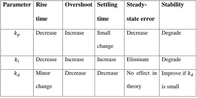
By introduction of PID controller we can control these above system dynamics

using tuning methods and thus determine various parameters. The effects of these

parameters on system response are shown in table below.

We can see that with increase in the value of , we get better steady state

stability as it reduces the steady-state error. The integral control can nullify the

steady state error but cost paid is that it makes the system sluggish. While above

two lead to oscillatory response initially, the derivative control makes the

overshoot within limit and also improves the settling time.

(21)

Table 2:-

Parameter Rise

time

Overshoot Settling

time

Steady-state error

Stability

Decrease Increase Small

change

Decrease Degrade

Decrease Increase Increase Eliminate Degrade

Minor

change

Decrease Decrease No effect in

theory

Improve if

is small

Effects of increasing control parameter independently

Table [2] shows how change in various gain parameters affects the response of the

system both transient and steady state.

THE 741 OPAMP

The OPAMP stands for operational amplifier. The opAmp is an amplifier with

some specific important characteristics. As the word amplifier suggests, the

function of an operational amplifier (op amp) is to amplify a voltage. However, the

operational amplifier does much more than that. It also functions as a buffer and as

a cascade which are two functions that enable simple circuits to be assembled into

complex circuits to create higher level functions which are called operations¾

(22)

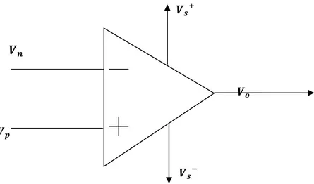
Op amps have five terminals that are important. The voltage that is amplified is the

difference between the voltage at the ‘+’ terminal and the voltage at the ‘-’

terminal , as shown in figure below. The amplified voltage is the output voltage

. Unlike the resistor and capacitor, which are both “passive” (unpowered)

devices, the opamp is an “active” device. Indeed, the op amp needs a voltage

supply for the amplification. The and the terminals are the positive and

negative supply voltages, respectively. The op amp schematic and the chip that

we’ll use are shown in figure below. Generally it is available in integrated chips.

The pin configuration of 741 IC is as shown below.

Offset unused

offset

Fig 4- Pin configuration of 741 opamp

1 8

2 7

3 6

(23)

Fig 5- Circuit symbol of an opamp

DATASHEET FOR LM741

Absolute maximum Ratings

TABLE 3:-

LM741A

LM741

LM741C

Supply Voltage ±22V ±22V ±18V

Power Dissipation 500 mW 500 mW 500 mW

Differential Input

Voltage

±30V ±30V ±30V

Input Voltage ±15V ±15V ±15V

Output Short Circuit Duration

Continuous Continuous Continuous

(24)

Temperature Range

Storage

Temperature Range

−65°C to +150°C −65°C to +150°C −65°C to +150°C

Datasheet for 741 IC

“Absolute Maximum Ratings “indicate the limits beyond which damage to the

device may occur. Operating Ratings indicate the conditions for which the device

is functional, but do not ensure specific performance limits. For operation at

elevated temperatures, these devices must be derated based on thermal resistance.

For supply voltages less than ±15V, the absolute maximum input voltage is equal

to supply voltage.

OPAMP REALISATIONS

SIGNAL BUFFER:-

It is a circuit configuration in which input equals output. The importance

of this circuit is that it isolates the input and output side. Since, the input current of

opAmp is 0, loading effect is 0. So, we can measure the actual input without error

due to loading. Its circuit diagram is shown below.

(25)

SIGNAL INVERTER:-

This circuit changes the polarity of the input signal with amplification and

the gain value is,

(12)

Fig7- signal inverter circuit

SIGNAL ADDER/SUMMER:-

This circuit helps in summing up various signals .Here, output voltage is given by

(26)

R

Fig 8- signal summer circuit

SIGNAL SUBTRACTOR/DIFFERENTIATOR:-

This circuit gives the difference of the two inputs given to the opamp circuit,

provided all the resistances should have same value as shown in the circuit below.

Here output signal is given as

(14)

R

R R

(27)

CHOICE OF CIRCUIT PARAMETERS

We need to initially determine the values of , and for a certain PID

controller. Since our plant is unknown we assume our plant to be anything

arbitrary and thus our controller should be tunable one.

We need a PID controller for 0<= <=100, 0<= <=10 and an arbitrary as per

requirement.

Firstly, we need to test each components of the controller viz., proportional,

integral and derivative terms separately and then integrate them together. So, we

assemble the components for the proportional controller. As 0<= <=100, we

chose our pot and ohms. We chose a 741 opAmp for this

purpose. Initially, we set up the board as shown in circuit diagram below.

100k pot Sine input

1kohm

Output

(28)

Then, we supplied a sinusoidal voltage wave from a function generator as input to

the controller circuit. The input and output waveforms were viewed in a CRO. The

results were noted and waveforms were traced in tracing paper. The experiment

was repeated by varying the values of using potentiometer. Results were viewed

and traced.

Now, we needed to do the same test with the derivative controller. Here, we

needed to supply a ramp input and check the output. Since, ramp signal cannot be

generated due to saturation, so, we used a triangular wave input to the controller.

As we required 0<= <=10, we use a 10 micro Farad capacitor, a 1K resistor and

a 1M pot for the purpose, as shown in below circuit diagram. Waveforms were

viewed in CRO and traced in tracing paper.

1M pot Triangular input

1kohm 10µF

Output

Fig 11- derivative controller

Next, we repeated the test for integral controller with circuit diagram as shown

(29)

small, resistance say 1kohm was put in series with the capacitor as shown in the

circuit diagram above.

Input given to the controller was a square wave. Output waveforms were viewed

and traced in a tracing paper. Results were obtained for different values of by

varying the potentiometer. The same was repeated by replacing the 1 micro Farad

capacitor with a 10 micro Farad capacitor.

1µF/10µF Square input

1M pot

Output

Fig 12- integral controller

Now, after performing these entire tests we move on to fabricate our PID

controller .The circuit diagram for the design is shown below. The components

used for whole process are shown in table below. The components are assembled

together and the connections were made as per circuit diagram on the bread board.

The supply voltages for the 741 opamps are not shown in the circuit diagram.

Supply voltage of ±15V was given to the IC’s. Then inputs were supplied using

function generator and the required waveforms were traced on the tracing paper.

Finally, after the testing the components were removed from the bread board and

(30)

100k 100k pot

100k Process 1k

100k 100k

output 10µF

Set point 1M pot

100k 100k

100k

1M pot 100k

1k 10µF

Fig 13- complete pid controller circuit

dedicated as input buffer, while one for output buffer. The process variable and set

point variable are given at the input and we get the same values of input at the

output terminals. Next, both the inputs are subtracted using another opamp IC

which uses four equal resistors of 100k each. This generates an error signal at its

output. The output of this is given to each of the individual controllers viz.,

proportional, integral and derivative. The controllers are nothing but three signal

inverters with two resistors in proportional control and one capacitor and one

resistor in both integral and derivative controls with their position exchanged in

each. The output of the three controllers is summed up using a summer circuit and

(31)

the whole control circuit from outside loads. The controls of the variables are

achieved using the three potentiometers as shown in figure. As we can see that

proportional term contains a 100 pot, derivative and integral terms contain 100M

pots, which is done in order to achieve required range of values of and .

In the derivative control, we find a small resistor of 1k. This is given in order to

save the capacitor from short circuiting because we now that uncharged capacitor

when connected to a voltage source acts like a short circuit initially. So, this

resistor limits the short circuit current.

TABLE 4:-

Sl. No

Components used

Quantity

1 OpAmps (741)

8

2 100k pot

1

3 1M pot

2

4 100k resistors

8

5 1k resistor

2

6 1microFarad capacitor

1

7 10microFarad capacitor 2

8 Soldering kit

-

9 Multimeter

-

10 CRO

-

(32)

12 Connecting wires

As required

13 Bread

board/proto

board

-

14 7815

2

15 Fan to fan connecter

As required

16 Berg strip

As required

Components used in fabricating PID controller

TEST RESULTS

The supply voltage given was ±18v through an adapter which was then converted

to ±15V using 7815. Then required test was performed. After performing the test

on proportional controller, it was found that the peak to peak value of sine

waveform got reduced with increase in the value of , and the waveform

approached a steady dc value with almost no ripples.

The output of the derivative controller was a square wave corresponding to a

triangular input as expected. The variation of had practically no effect on the

waveform except that there was a slight variation in duty cycle for variation of

from 0 to 10.

The output of integral controller showed both positive and negative peaks when a

1 micro Farad capacitor was used. When the capacitor was replaced by a 10 micro

Farad capacitor the output waveform was similar to input wave with a large rise

(33)

CONCLUSION

It was found that the proportional controller reduces the transients to an

appreciable extent and thus, should have high value. The derivative controller

acts on the rate of change of input and thus converts the triangular wave to a

square wave. It is very sensitive to changes or variations in the input.

As far as integral controller was concerned, it had a slow rise and decay time

making system sluggish. The output waveforms were found almost as expected

and thus, the analog pid controller was fabricated finally.

REFERENCES

1] Nagrath, I.J. and Madan, Gopal, Control system engineering, 5th Edition, New

Age International Publisher, 2007

2] Bennett, Stuart (1993), A history of control engineering, (1930-1955), IET.

P.48. ISBN 978-0-86341-299-8

3] Ang, K.H., Chong, G.C.Y., and Li, Y. (2005). PID control system analysis,

design, and technology, IEEE Trans Control Systems Tech, 13(4), pp.559-57

A THESIS SUBMITTED IN PARTIAL FULFILMENT OF THE REQUIREMENTS FOR THE DEGREE OF

ANALOG FABRICATION OF PID

CONTROLLER