Abstract
The problem of model predictive control (MPC) under parametric uncertainties for a class of nonlinear systems is addressed. An adaptive identifier is used to estimate the pa-rameters and the state variables simultaneously. The algorithm proposed guarantees the convergence of parameters and the state variables to their true value. The task is posed as an adaptive model predictive control problem in which the controller is required to steer the system to the system setpoint that optimizes a user-specified objective function.
The technique of adaptive model predictive control is developed for two broad classes of systems. The first class of system considered is a class of uncertain nonlinear systems with input to state stability property. Using a generalization of the set-based adaptive estimation technique, the estimates of the parameters and state are updated to guarantee convergence to a neighborhood of their true value.
Table of Contents
Chapter 1 Introduction
1.1 Introduction 1
1.2 Organization of the Dissertation 2
Chapter 2 Literature Review
2.1 Technical Preliminaries 4
2.2 Parameter Estimation in Nonlinear Systems 10
2.3 Real-time Optimization 12
2.4 Summary 17
Chapter 3 Adaptive Receding Horizon Control Of Input Constrained Nonlinear Systems
3.1 Introduction 18
3.2 Mathematical Background 19
3.3 Problem Description 20
3.4 Adaptive Model Predictive Control 21
3.5 Estimation of Uncertainty 24
3.6 Simulation Examples 26
3.7 Summary 29
Chapter 4 Passivity Based Parameter Estimation in Adaptive Control of Nonlinear Systems
4.1 Introduction 30
4.2 Mathematical Background 30
4.3 Problem Description 31
4.4 Infinite Time Parameter Identification 32
4.5 Finite Time Parameter Identification 35
4.6 Supporting Example 36
4.7 Summary 36
Chapter 5 Adaptive Predictive Control of
Nonlinear Systems: An Application to a CSTR system
5.1 Introduction 38
5.2 Problem statement 39
5.3 Parameter Identification Algorithm 39
5.4 Adaptive Predictive Control Scheme 40
5.5 CSTR Dynamics 42
5.6 Summary 43
Chapter 1 Introduction
The problem of parameter and state estimation of a class of nonlinear systems is ad-dressed. An adaptive identifier and optimal control problem are used to estimate the param-eters and control system states variables simultaneously. The proposed method is derived using a new formulation. An algorithm is developed to update these sets using the available information. The algorithm proposed guarantees the convergence of parameters and the state variables to their true value.
The technique of estimation is applied to two broad classes of systems. The first involves a class of continuous time nonlinear systems subject to bounded state and input systems with constant unknown parameters. Using the proposed set-based adaptive estimation, we can steer system optimally to the origin. The formulation provides robustness to parameter estimation error. The parameter uncertainty set and the uncertainty associated with an auxiliary variable is updated such that the set is guaranteed to contain the unknown true values. The second class of system considered is a class of nonlinear systems with ISS-CLF stability condition. Using a generalization of the set-based adaptive estimation technique proposed, the estimates of the parameters and state are updated to guarantee convergence to a neighborhood of their true value. To study the practical applicability of the developed method, the estimation of state variables and parameters in a stirred tank process has been performed. The results demonstrate the ability of the proposed techniques to estimate the state variables and parameters of the uncertain system.
1.1 Introduction
rate in bioreactors are the examples of process parameters. Information on the parameters of a process provides a better understanding of the process dynamics and also allow for the development of an accurate and representative models of process.
In practice, due to inadequacy of available sensors or operational limitations, some of the es-sential process state variables cannot be measured frequently. In addition important process parameters may have to be estimated from available measurements. In such cases, estimates of the inaccessible, but essential, state variables and parameters of the process are usually obtained by employing state and parameter estimation methods. Many techniques exist for the estimation of states for a variety of classes of dynamical systems that can achieve accurate state estimates in a variety of conditions. However, these techniques rely on the knowledge of the system parameters. Uncertainty in the model parameters for instance can generate (possibly large) bias in the estimation of the unmeasured state variables. In cases where large uncertainties of the process parameters exist, it is imperative to use techniques that are able to combine state observation with parameter estimation.
The motivation for this research arises from the need to develop reliable state and parame-ter estimation methods that are capable of providing continuous and accurate estimates of inaccessible state variables and parameters of a nonlinear process in a presence of exogenous disturbance and running the system to the origin which is frequently encountered in practice.
1.2 Organization of the Dissertation
Chapter 2: Chapter 2 is divided into two parts. First, the technical preliminaries re-quired to develop the parameter and state estimation methodology proposed in Chapter 3 are introduced. The topics include Persistence of Excitation (PE), Lyapunov Stability, Projection Algorithm, Observability, State Observers and Adaptive identifiers. The second section contains a review of the past and recent works in the field of real time optimization and model predictive control of nonlinear systems.
parame-ters and the state variables are updated to guarantee convergence. A simulation example is used to illustrate the developed procedure and ascertain the theoretical results.
Chapter 4: In this chapter, we consider the problem of parameter identification and state estimation of a continuous-time nonlinear system subject to unknown parametric un-certainty. The formulation is developed to provide robustness to parameter estimation error. The uncertainty associated with an auxiliary variable defined for state estimation is updated such that the set is guaranteed to contain the unknown true values. A simulation example is used to illustrate the developed procedure and ascertain the theoretical results. After convergence of the variables to the true values, a model based predictive control is defined to run the system simultaneously to the origin.
Chapter 5: Based on the results in Chapter 4, the estimation technique is applied to a mixing tank problem. The developed method is used to estimate state and parameters of the experimental process. The estimation routine employed guarantees convergence of state and parameters to their true values.
Chapter 2 Literature Review
The design methodology for simultaneous parameter and state estimation and optimal control of class of a nonlinear systems is largely developed from the concepts of linear sys-tem theory, parameter identifiers, projection algorithm and adaptive predictive control. In this chapter, these concepts are briefly introduced for the understanding of this thesis work. The detailed discussion regarding the relationships between the concepts are discussed in Chapter 3. This chapter also summarizes the recent and early works by researchers active in robust adaptive predictive control techniques that are of importance in relation to this thesis.
2.1 Technical Preliminaries
2.1.1 Persistence of Excitation
The concept of persistent excitation (PE), when it arose in the 1960s in the context of system identification. The term PE was coined to express the property of the input signal to the plant that guarantees that all the modes of the plant are excited. In the late 1970s, it became clear that the concept of PE also played an important role in the convergence of the controller parameters to their desired values. Recent work on robustness of the adaptive systems in the presence of bounded disturbance, time-varying parameters, and un-modeled dynamics of the plant revealed that the concept of PE is also intimately related to speed of convergence on the parameters to their final values, as well as the bounds on the magnitudes of the parameter errors. In both linear and nonlinear adaptive systems, parameter convergence is related to the satisfaction of persistence of excitation condition, which can be defined in the continuous time as follows.
Definition 2.1.1: [Krstic et. al, 1995] A vector functionφ : is said to be persistently exciting if there exist positive constants α1,α2 and T0 such that
α1I ≥ Z t+T0
t
φ(τ)φ(τ)T ≥α2I,∀t ≥0 (1)
re-of matrix φ(τ)φ(τ)T should attain full rank over any interval of some length T
0 or in other words, (1) requires that φ(t) varies such that the integral of the matrix φ(τ) is uniformly positive definite over any time interval [t, t+T0]. The properties of PE signals as well as various other equivalent definitions and interpretations are given in the literature. In adap-tive linear systems, the PE condition is converted to the sufficient richness (SR) condition on the reference input signal. Necessary and sufficient conditions for parameter convergence are then developed in terms of the reference signal. A popular result implies that expo-nential convergence is achieved whenever the reference signal contains enough frequencies, i.e., whenever the spectral density of the signal is nonzero in at least nθ points, where nθ is the number of unknown parameters in the adaptive scheme. Otherwise, convergence to a characterizable subspace of the parameter space is achieved. Despite the fact that the theory of parameter convergence for linear systems is well established, very few results are available for nonlinear systems. This is mainly because the familiar tools in linear adaptive control cannot be directly extended to nonlinear systems. In most of the available results, stability and performance properties are proved by assuming that a vector function, which depends on closed-loop signals is persistently exciting. However, the means of verifying this PE con-dition a priori for a given nonlinear system remains an open problem, in general. In [Lin and Kanellakopoulos, 1998], a procedure is provided for determining a priori whether or not a specific reference signal is sufficiently rich for a specific output feedback nonlinear system, and hence whether or not parameter estimates will converge. Nevertheless, the main result in [Lin and Kanellakopoulos, 1998] is that the presence of nonlinearities in the plant usually reduces the SR condition requirement on the reference signal and thus enhances parameter convergence.
2.1.2 Lyapunov Stability
explicitly integrating the ordinary differential equations. In addition, the Lyapunov analysis is applicable to continuous-time and discrete-time systems, linear and nonlinear systems, time-invariant and time-varying systems. From the classical theory of mechanics, a vibratory system is stable if its total energy is continually decreasing until an equilibrium state is reached. A physical example that illustrates this concept is a simple pendulum in which the equations of motion described by the forces acting on the system, vanish at steady state [Khalil, 2002]. The method of Lyapunov, is based on the following behavior. If the system has an asymptotically stable equilibrium state, then the stored energy of the system decays with increasing time until it finally reaches its minimum value at the equilibrium state. For a general system, however it is not simple to describe its dynamics through an energy function. To overcome this difficulty, the Lyapunov function which acts as a fictitious energy function, was introduced [Ogata, 1987].
Lyapunov stability analysis plays an important role in the stability analysis of dynamical systems described by ordinary differential equations. The Lyapunov function, denoted by V (.), is a scalar, positive definite function. It is generally assumed to be continuous with continuous partial derivatives. When taken along the systems trajectory, the time derivative of the Lyapunov function is negative definite or negative semidefinite. These desired prop-erties of the Lyapunov function can be formally stated in the stability theorem described by [Khalil, 2002] for a non-autonomous system.
Theorem 2.1.2.1. [Khalil, 2002] Consider the non-autonomous system
˙
x(t) = f(t, x(t)) (2)
where f : [0,∞)×D → Rn is piecewise continuous in t and locally Lipschitz in x(t) on [0,∞)×D, system (2) at t = 0 and D={x(t)∈Rn| ||x(t)||< r}. Let V : [0,∞)×D→R be a continuously differentiable function such that,
α1(||x(t)||)≤V(t, x(t))≤α2(||x(t)||) (3)
˙
V(t, x(t)) = ∂V ∂t +
∂V
∂xf(t, x(t))≤0 (4) Z t+
∀t ≥ 0,∀x(t) ∈ D, for some , where α1(·) and α2(·) are class K functions defined in [0, r) and φ(τ, t, x(t)) is the solution of the system that starts at (t, x(t)). Then, the origin is uniformly asymptotically stable.
If all the assumptions hold globally and α1(·) belongs to classk∞ then the origin is globally uniformly asymptotically stable.
Now that the stability considerations based on Lyapunov theory are defined, the next step consists of finding a convenient Lyapunov function to design the adaptive updating laws, such that Theorem 2.1.2.1 is satisfied.
2.1.3 Projection Algorithm
It is important to mention that, in general, the parameters that characterize a system, have a physical meaning and are bounded above and/or below. For this reason, it is desired to constrain the parameter estimates to lie inside a bounded set. An effective method for keeping the parameter estimates within some defined bounds is to use a projection algorithm. In many practical problems where θ represents the parameters of a physical plant, we may have some a priori knowledge as to where θ is located inRn. This knowledge usually comes in terms of upper or lower bounds for the elements ofθor in terms of a well defined subset of Rn, etc. Using this a priori information, adaptive laws can be designed that are constrained to search for estimates of θ in the set where θ is located. Intuitively such a procedure may improve the convergence and reduce the time taken in convergence when initial values of the parameter is chosen to be far away from the unknownθ . In [Krstic et al., 1995], a projection operator is defined for the general convex parameter set Π.
Consider a convex set Π = {θˆ∈ Rp|P(ˆθ) ≤ }, , where the convex function P : Rp → R is assumed to be smooth. The set Π is the union of the set Π = {θˆ∈ Rp|P(ˆθ) ≤ 0} and a boundary around it. The interior of Π is denoted by ˙Π, and ∇θˆP represents an outward normal vector at ˆθ∈∂Π. The projection operator is defined as follows
proj(τ) =
τ if ˆθ ∈Π or˙ ∇ˆθPTτ ≤0; (I−c(ˆθ)Γ∇θP∇ˆ θP Tˆ
ˆ
θPT∇θPˆ )τ if ˆθ∈Π\Π and˙ ∇ˆθPTτ >0;.
(6)
Here, Γ belongs to G of all positive definite symmetric p×p matrices and τ is the vector of nominal update laws that is, in the absence of the projection algorithm the update law
˙ˆ θ =τ.
The properties of the projection operator, P roj{τ,θ,ˆ Γ}, are given by
1. The mapping P roj :Rp×Π×G→Rp is locally lipschitz in its arguments τ,θ,ˆ Γ. 2. P roj{τ}TΓ−1P roj{τ} ≤τTΓ−1τ,∀θˆ∈Π
. 3. Let Γ(t)τ(t) be continuously differentiable and
ˆ
θ =P roj{τ},θˆ(t)(0) ∈Π
Then, on its domain of the definition, the solution ˆθ(t) remains in Π.
The adaptive laws with the above projection modification retain all the properties estab-lished in the absence of the projection and guarantee that ˆθ∈Π,∀t≥0 provided ˆθ(0)∈Π.
2.1.4 Observability
Consider a continuous time linear system of the form
˙
x=Ax+Bu (7)
y=Cx (8)
where x ∈ Rn is a state vector, u ∈ Rn is the control input, y ∈ Rn are the outputs, and matrices, A,B and C are of appropriate dimensions. Observability is a property of dynamical system, first introduced by [Kalman, 1960]. This property is meant to express the availability of measurement data with respect to ones ability to reconstruct or make inferences regarding the values of unmeasured state variables.
Definition 2.1.4.1: A linear continuous time system given by (7,8) is observable if for any initial state x0 and some final time t, the initial state x0 can be uniquely determined by knowledge of the inputs u and outputs y for all time t.
that can occur. If a system is observable, then its initial state can be determined. If the initial state is known, then values of the states at any time can be calculated. Hence, observability implies that values of the state at any time are fully reconstructible as long as the inputs and outputs are known exactly. Observability can be checked by a matrix rank test performed on the systems observability matrix.
Theorem 2.1.4.1: The continuous time LTI system (7,8) is observable if and only if the observability matrix is defined by
O(C, A) = [CT,(CA)T,· · · ,(CA(n−1))T]T (9)
is of rank n.
The concept of observability is central to the design of state observers and state estima-tors, which are discussed in the next section.
2.1.5 State Observers
Many nonlinear control design and adaptive system techniques assume state feedback; this implies that all the state variables are measured and are available for feedback. In practice, this is not always true, either for economic or technical reasons, such as sensor failures. In most cases,only a subset of the state variables are available for measurement. Intuitively, we want to use the measured states or outputs of the system and extend the state-dependent techniques to output-dependent techniques for system design. The idea is similar to what has been widely applied in LTI systems, i.e., build an observer that yields asymptotic esti-mates of the system state based on the output of the system, and then update the control/ adaptation law using on-line estimation of the unmeasured states. In control theory, a state observer is a dynamical system whose outputs are the estimates of the state variables of the system [Ioannau and Sun, 1996]. The main criterion that observers must satisfy is that the estimation error ˜x(t) = (x(t)−xˆ(t)) tends to zero in the limit as t → ∞ where ˆx(t) is the estimate of the state x(t) at time t. If the dynamics of the plant give rise to a linear time-invariant system, then there exists an estimator of the form
ˆ
x(t) = Axˆ(t) +L(y−yˆ) +Bu (10)
ˆ
which guarantees convergence of the state estimation error to zero, provided that the plant is observable. The observer given by Eqs. (2.5a) and (2.5b) is referred to as a Lu-enberger observer [Ioannau and Sun, 1996]. The matrix L is designed so that the matrix (A−LC) is stable, which ensures the stability of the observers error dynamics. In fact, the eigenvalues of (A −LC), and, therefore, the rate of convergence of ˜x(t) to zero can be arbitrarily chosen by designing L appropriately. Therefore, it follows that ˆx(t) → x(t) exponentially fast as t → ∞, with a rate that depends on the matrix (A−LC). This result is valid for any matrix A and any initial conditionx(0) as long as (C, A) is an observable pair.
2.1.6 Adaptive Identifiers
The adaptive identifiers represent a class of real time parameter estimation schemes that are used to estimates (typically) slow time-varying parameters of dynamical systems. Under suitable conditions, these identifiers can guarantee convergence of the estimated parameters to the unknown parameter values. The design of such scheme includes the selection of plant input so that a certain signal vector, is PE. Adaptive identifier designs are natural extension of observer design for linear time invariant (LTI) systems with unknown parameters. When the parameters of the system are unknown, an adaptive identifier is designed to estimate the parameters of the dynamical system. This was first accomplished in [Kreisselmeier, 1977; Kudva and Narendra, 1973]. Traditionally, an adaptive identifiers consists of a state prediction subject to parameter estimations and a parameter update law. Different repre-sentations have been discussed in detail for LTI systems [Ioannau and Sun, 1996; Narendra and Annaswamy, 1989; Sastry and Bodson, 1989]. Basic methods used to design adaptive laws include Lyapunov-based design, gradient methods, and recursive least squares meth-ods. Subsequently alternative techniques have been generalized to the design of adaptive observers for nonlinear systems, linear time-varying systems and systems with disturbances. Adaptive laws only become parameter identifiers if the input signal u has to be chosen to be sufficiently rich so that the regressor vector φ is PE.
2.2 Parameter Estimation in Nonlinear Systems
Guay, 2008], the authors considered a system with exogeneous disturbances and showed that parameter convergence can be guaranteed under certain conditions of persistency of excitation condition. The authors proposed a novel set-based adaptive estimation with an appropriate adaptation law for the unknown parameters. The proof of the convergence of the estimates to their true values is achieved using Lyapunov theories.
2.3 Real-time Optimization
One of the key challenges in the process industry is how to best operate the plant under different conditions such as feed compositions, production rates, energy availability, feed and product prices that changes all the time. Real-time optimization (RTO), which refers to the online economic optimization of a process plant, is a widely employed technology to meet this challenge. RTO attempts to optimize process performance (usually measured in terms of profit or operating cost) thereby enabling companies to push the profitability of their processes to their true potential as operating conditions change. The popular RTO is based on the assumption that model and disturbance transients can be neglected if the op-timization execution time interval is long enough to allow the process to reach and maintain steady-state. A typical RTO system includes components for steady-state detection, data acquisition and validation, process model updating, optimization calculations and optimal operating policies transfer to advanced controllers.
2.3.1 Model Predictive Control
Model predictive control (MPC) or receding horizon control (RHC) is a family of control that utilizes a process model along with cost factors and optimum target operating point to calculate process control moves that drives the plant to the most economic constraints while ensuring stable operation. The control technique has proven to be extremely successful in the process industry. Linear (and nonlinear) model predictive control remains the industry standard with increasing number of reported applications and significant improvements in technical capability [Camacho and Bordons, 1995]. Consider the time-invariant nonlinear system of the form
˙
subject to the pointwise state and input constraints x(t) ∈ X ⊂ Rnx and u(t)∈ U ⊂ Rnu, respectively. The vector fieldf :Rnx×Rnu →Rnx satisfiesf(0,0) = 0, the set U is compact, X is connected and (0,0)∈(X, U).
MPC algorithms optimize the future plant behaviour and satisfy the given constraints by solving the following finite horizon open loop optimal control problem:
minup J = Z t+T
t
L(xp(τ), up(τ))dτ +W(xp(t+T)) (13)
s.t. ˙xp =f(xp(τ), up(τ)), xp(t) =xt xp(τ)∈X, u(τ)∈U
xp(t+T)∈Xf
where (.)p denotes the predicted variables (internal to the controller). The stage cost L(xp, up) is a semi-definite positive function. The terminal penaltyW(xp(t+T)) and termi-nal constraint xp(t+T)∈Xf are included for stability considerations.
At each time step, the solution to the optimization problem is found over a certain predic-tion horizon, T, using the current state of the plant or its estimate as the initial state. The optimization yields an optimal control sequence and the first control action is implemented on the plant until the results of the next update are available.
Model predictive control is part of the multi-level hierarchy of control structure. Using a numerical optimization scheme as an integral part of the structure allows great flexibility, especially concerning the incorporation of constraints. Though such optimization over a finite horizon does not guarantee stability and performance, considerable research has been devoted to address these shortcomings. Linear MPC theory and related issues such as closed-loop stability and online computation have been well studied and characterized [Magni, 2001, Mayne, et. al, 2000]. Over the past few years, nonlinear model predictive control (NMPC) schemes with some favorable properties have been developed. The theory related to stabil-ity of state and output feedback NMPC have reached a point of relative maturstabil-ity, see for example [ Chen and Allgower 1998, Findeisen et. al. 2003] for review.
2.3.2 Closed-loop Stability of NMPC Based on Nominal Model
given below [Findeisen et. al. 2003].
Criterion 2.1 The terminal penalty function W : Xf → R≥0 and terminal set Xf are such that there exists a local feedback kf :Xf →U satisfying
1. 0∈Xf ⊂X, Xf is closed
2. W(x) is positive semi-definite and continuous with respect to x∈Rnx 3. kf(x)∈U,∀x∈Xf
4. Xf is positively invariant under kf
5. L(x, kf(x)) + ∂W∂xf(x, kf(x))≤0,∀x∈Xf
The conditions are primarily concerned with the selection of terminal regionXf and ter-minal penalty termW(·). Condition 5 requiresW(·) to be a control Lyapunov function, over the (local) domain Xf , and dissipates energy at a rate L(x, kf(.)). This criterion, which is able to re-cast many of the available MPC frameworks with guaranteed stability, provides a means of checking whether a given MPC scheme guarantees stability a-priori. Stability is proven by showing strict decrease of the optimal cost function J∗, which is a Lyapunov function for the closed-loop system. The domain of attraction for the controller is the set where the optimization problem is feasible.
2.3.3 NMPC for Uncertain Systems
The quality of the model used in MPC is crucial to the performance of the controller. The as-sumption that the prediction model is identical to the actual model is unrealistic. Although, due to the receding horizon policy, a standard implementation of MPC using a nominal model of the system dynamics exhibits nominal robustness to sufficiently small disturbances [Camacho and Bordons, 1995], such marginal robustness guarantee may be unacceptable in practical applications. Present model/plant mismatch and disturbances must be accounted for in the computation of the control law to achieve robust stability.
the potential to improve system performance as it updates the model online based on mea-surement data. However, practical applications of adaptive controllers are limited by the conflicting objective of parameter estimation and control. This could lead to a worse tran-sient performance than a non-adaptive controller when poor estimates are used. Moreover, the controller may induce large transient oscillations in an effort to improve the estimation quality.
2.3.4 Robust Model Predictive Control
Robust techniques have been employed in MPC designs to reduce the sensitivity of the controller to uncertainty. Consider the following uncertain system
˙
x=f(x, u, ν) (14)
where ν(t) ∈ D represents any arbitrary bounded uncertainty or disturbance signal. Many robust MPC techniques have been proposed to stabilize the uncertain system for all possible realization of the disturbanceν(t)∈D. These include approaches based on nominal prediction [Magni et al 2003] and those based on min-max or worst-case techniques [Adetola and guay 2008].
The nominal based approach in [ Marruedo et. sl. 2002] uses global Lipschitz constants to compute 11 worst-case upper bound on the distance between a solution of the actual uncer-tain model and the nominal model. These bounds are then used to redefine the terminal region and constraints in a way that guarantees robust feasibility of the closed-loop system. The controller proposed in [Limon et. al. 2005] is based on the concept of reachable sets. The approach uses a local procedure to approximate the sets that contain the predicted evolution of the uncertain system for all possible uncertainties. Then, a dual mode MPC strategy is proposed to robustly stabilize the system. The methods based on nominal pre-diction have similar computational complexity with standard NMPC but exhibit a higher level of conservatism.
(in most cases) since the problem size grows exponentially with the size of the problem data. In general, robust MPC is designed to meet control specifications for the ” worst case” un-certainty. This approach may not always achieve optimal performance, in particular, if the worst case scenario rarely exists. Other approaches, such as adaptive control may yield a better performance.
2.3.5 Adaptive Model Predictive Control
Adaptive MPC is an attractive way to handle static uncertainties that can be expressed in the form of constant unknown model parameters. While a few results are available for linear adaptive MPC [Mayne et. al., 2000], only a small amount of progress has been made in developing adaptive NMPC schemes. Consider the parameter-affine nonlinear system of the form
˙
x=f(x, u, θ), f(x, u) +g(x, u)θ, (15) =f(x) +g1(x)u+g2(x)θ (16) The result in [Adetola and Guay 2004], implements a certainty equivalence nominal-model MPC feedback to stabilize this system subject to an input constraint u∈U. Assuming the availability of the state vector ˙x , the identifier guarantees parameter convergence when an excitation condition is satisfied. It is only by assumption that the true system trajectory remains bounded during the identification phase. Moreover, there is no mechanism to en-hance the satisfaction of the PE condition and thereby decrease the identification period. In general, the design of adaptive nonlinear MPC schemes is very challenging because the ” separation principle assumption” widely employed in linear control theory is not applicable to a general class of nonlinear systems, in particular in the presence of constraints. More-over, it is difficult to guarantee state constraints satisfaction in the presence of an adaptive mechanism. A true adaptive nonlinear MPC algorithm must address the issue of robustness to model uncertainty while updating the systems parameters.
constraints. The parameterization of the feedback MPC policy in terms of the uncertainty set and the underlying min-max feedback MPC used in the study make the controllers com-putation very challenging. The result can be viewed as a conceptual result that focus on performance improvement rather than implementation. The idea of coupling set-based iden-tification with robust control calculations was extended in [DeHaan et. al. 2007] to a less computationally complex robust-MPC framework.
2.4 Summary
Concepts and principles of parameter and state estimation are reviewed in this chapter. An overview of recent developments in parameter and state estimation of systems has been pre-sented.
Also, we have reviewed principle of model predictive control strategy and talked on robust model predictive control and adaptive model predictive control strategies.
Chapter 3
Adaptive Receding Horizon Control
Of Input Constrained Nonlinear Systems
In this chapter a method for adaptive receding horizon control of nonlinear systems is
introduced. Asymptotically stability and optimality in run of the closed loop systems in the
presence of parametric uncertainty is obtained employing input to state stabilizing
Lyua-punov control functions.
3.1 Introduction
Receding Horizon Control (RHC), usually called Model Predictive Control (MPC) has long
been preferred tool for advanced control applications. The relative ease with which
con-strained can be incorporated has attracted great deal of interest both in academia and
industry. They arise in a range of classical, as well as certain emerging, engineering
appli-cations [Qin and Badgwell, 2003] . Despite significant advances in this area still there is an
obstacle that an accurate knowledge of the model is instrumental. As a result, its application
remains constrained to processes with well-established model dynamics. However, in
gen-eral, most physical systems possesses parameter uncertainties and unmeasurable parameters
[Krstic et. al., 1995] and mechanisms to upgrade the unknowns or uncertainty parameters
are highly appealing [Adetola and Guay, 2004].
The main goal of this chapter is to report an online adaptive integrated parameter
estima-tion and RHC control method for input constrained nonlinear systems. To date, very few
adaptive nonlinear RHC schemes are developed for nonlinear systems [Peter and Guay 2007,
Adetola and Guay, 2004].
In the present work, we report a stable adaptive receding horizon scheme for parametric
uncertain systems. The adaptive receding horizon control scheme developed in this report is
based on the knowledge of an ISS-control lyapunov function (ISS-CLF) for the nonlinear
sys-tem. The structure of the chapter is as follows. First, we review some technical background
and then introduce and formulate the problem, thereby an Adaptive RHC+CLF problem is
strategy be used which is stated in Section 4. Finally we prove asymptomatically stability
of the proposed scheme.
3.2 Mathematical Background
Consider the function W :D×R+ →R. Assume 0∈D and W(x, t) is continuous and has
continuous partial derivatives to all its arguments.
Definition 3.2.1: W is said to be positive definite in D if
W(0, t) = 0, ∀t∈R+
W(x, t)>0, ∀x6= 0, x∈D.
Definition 3.2.2: W(x, t) is said to be decrescent in D if there exist a positive definite function V(x) such that
|W(x, t)| ≤V(x), ∀x∈D
Definition 3.2.3: W(x, t) is radically unbounded if
|W(x, t)| → ∞ as |x| → ∞ uniformly in t
Definition 3.2.4: Consider the system
˙
x=f(x, t),
f : D×R+ → Rn Where f is point-wise continuous in t on D×[0,∞]. x = 0 ∈ D is an
equilibrium point if
f(0, t) = 0,∀t≤t0.
Theorem 3.2.1: If in a neighborhood D of x=0 there exists functionW(·,·), D×[0,∞)→R
such that
i ) W(·,·) is positive definite, and,
ii) The derivation of W(·,·) along any solution of system f(x,t) is negative semi definite in
D, then,
This equilibrium point is stable and W(·,·) is called a lyapunov function.
Theorem 3.2.2: If in a neighborhood D of x=0 there exists functionW(·,·), D×[0,∞)→R
such that
i) W(·,·) is positive definite and decrescent, and,
ii) The derivation of W(·,·) is negative definite in D, then,
The equilibrium state is uniformly asymptotically stable.
Theorem 3.2.3: If there exist function W(·,·), D×[0,∞)→R such that i) W(·,·) is positive definite, decrescent and radically unbounded, and,
ii) The derivation of W(·,·) is negative definite for ∀x∈Rn, then
The equilibrium state is uniformly asymptotically stable.
Definition 3.2.5 : A continuous functionα(r) defined overr ∈[0, a] is said to belong to class
K if it is strictly increasing and α(0) = 0. It belongs to class K∞ if a =∞ and α(r) → ∞
as r→ ∞.
Definition 3.2.6 : A continuous functionβ : [0, a)×[0,∞)→[0,∞) is said to belong to class
KL if for any fixed s, the mapping β(r, s) belong to class K respect to r, and for any fixed r,
the mapping β(r, s) is decreasing respect to s, and β(r, s)→0 as s→ ∞.
Consider the system
˙
x=f(t, x, u)
where f : [0,∞]×Rn×Rm →Rn is piecewise continuous in t and locally litschitz in x and
u. The input u(t) is piecewise continuous function of t for all t≥0.
Definition 3.2.7: The system defined above is said to be input-to-state stable if there exist a
KL functionβ and a class K function γ such that or any initial state x(t0) and any bounded
input u(t), the solution x(t) exists for allt≥t0 and satisfies
|x(t)| ≤β(|x(t0), t−t0|) +γ(supτ∈(t0,t)(|u(τ)|))
3.3 Problem Description
We consider the nonlinear system,
˙
where f(x), F(x) and g(x) are smooth. For simplicity we consider f(0) = 0, F(0) = 0 so
that x= 0 is the equilibrium of the uncontrolled system.
Definition 3.1: A smooth positive definite radically unbounded functionV :Rn→R + is
called an ISS-control Lyapunov function (ISS-CLF) for eq(1) if there exist class K functions
α1, α2 and a class K∞ functionρ such that α1(kxk)≤V ≤α2(kxk) and the following holds
for all x6= 0 and all d∈Rr
kxk ≥ρ(kdk)
infu∈Rm{
∂V
∂x[f(x) +P(x)d+g(x)u]}<0. (2)
Note 3.1: The existence of an ISS-CLF guarantees that the nonlinear systems eq(1) is input to state stable with respect to the disturbance input d.
In this chapter we consider nonlinear systems of the form
˙
x=f(x) +P(x)θ+g(x)u, (3)
where x ∈ Rn and u ∈ Rm are systems measurable states and control inputs respectively,
θ ∈ Rp is the vector of unknown constant parameters. f(x) : Rn → Rm is a smooth
vec-tor function,P(x) :Rn →Rm×p andg(x) :Rn→Rm×mare smooth matrix valued functions.
3.4 Adaptive MPC
Computation of optimal input control action in model predictive control greatly relies on the
knowledge of parameter estimates, however, since there is no guarantee that the parameter
estimations approach their true value, the existence of offset is inevitable. The scheme
presented here ensures the robust stability of the controller to the estimation errors; Fist, we
develop a receding horizon controller based on the known ISS-CLF function to stabilize the
nonlinear system, and then an adaptive estimation procedure is developed to estimate the
parameters. Combination of the two schemes globally asymptotically stabilizes the origin of
the closed loop system. We define the unknown parameter estimation error
˜
where ˆθ are the assumed known parameter estimates and use the substitution of P(x)θ =
P(x)ˆθ+P(x)˜θ to rewrite the eq(3) as,
˙
x=f(x) +P(x)ˆθ+g(x)u+P(x)˜θ, (4)
For this system it is supposed that an ISS-CLF function, say V, is known. The problem of
determining an ISS-CLF for constrained systems has become the focus of research recently
and considerable progress has been reported in [Primbs, 1999]. Based on the available
ISS-CLF V we can introduce the following pointwise min-norm problem,
min uTu (5)
subject to V˙ ≤ −σ(x(t))ˆ (6)
with ˆσ(x(t))>0.
Since the input is unbounded, the stability constraint may make the problem infeasible for an
arbitrary choice of−σ(x(t) therefore its value must be properly chosen to avoid infeasibility.ˆ
We propose to accomplish this by solving the following optimization problem in u and ψ:
min uTu+λψ2 (7)
subject to V˙ ≤ −σ(x(t)) +ψ (8)
ψ ≥0 (9)
−σ(x(t)) +ψ ≤0 (10)
and set,
ˆ
σ(x(t)) =σ(x(t))−ψ (11)
with λ >0 a design parameter to be chosen. The other design parameter is σ which can be
chosen with lesser restrictions. We choose it based on the Sontag’s unconstrained formula,
σ =qa2+q(x)kbk2 (12)
where a = ∂V∂xf + ∂V∂xP(x)ˆθ+k∂V ∂xPkρ
−1(kxk), b = ∂V
∂xg and q(x) is some positive definite
The new re-formulated problem can be looked at as a point-wise min-norm problem in which
the objective function contains the penalty term λψ2, which is used to soften the constraints
and avoid the infeasibility. For each arbitrarily large but finite λ, this problem is always
feasible due to the existence of the ISS-CLF function V, (see eq (2)).
Lemma 3.4.1.: Let (u∗;ψ∗) be the optimal solution of the problem (5)-(6) for any given state x(t); then u∗ is also the optimal solution of (7)-(8) with ˆσ(x(t)) =σ(x(t))−ψ∗.
Proof: The proof is similar to that of Lemma 7.3.1. in [Primbs, 1999].
The implication of Lemma 1 is that allows us to always refer to the point-wise min-norm
problem (5)-(6), even though the problem (7)-(8) is effectively solved in order to obtain
a feasible solution. By determining a feasible ˆσ for the constrained point-wise min-norm
problem, we extend formulations for an Adaptive RHC+CLF scheme, given by,
minuJ =
Z t+T
t
q(x(τ), u(τ))dτ (13)
subject to
˙
x=f(x) +P(x)¯θ+g(x)u (14)
¯
θ= ˆθ (15)
V(x(t+T))≤V(xiss(t+T)) (16)
˙
V ≤ −σ(x(t))ˆ (17)
where xiss(t+T) is the state prediction for the model subject to the min-norm based
con-troller problem starting at the current state x(t) with the current parameter estimation ˆθ(t).
In RHC+CLF formulation the unknown parameter ¯θ in eq (15) replaces with the last
esti-mated parameter value. The optimizer computes the required control moves over prediction
horizon T. u(k|k)is implemented on the plant form the time step k to k+ 1 and then new
estimates of the unknown parameter ˆθ(k) is obtained from the parameter update law. The
prediction and control horizons are shifted forward by one step and a new optimization
prob-lem is solved at time k+ 1 and the procedure repeats by the end of the control horizon.
Notice that, in the formulation (13)-(17), ˆθ is supposed to be constant over the interval
remainder we study stability of RHC+CLF scheme to design parameter update law θ.˙ˆ
3.5 Estimation of Uncertainty
Let x∗(τ) be the state trajectory resulting from the proposed RHC+CLF scheme. Consider
the function,
W = 1 T
Z t+T
t
V(x∗(τ))dτ (18)
This function is positive definite and radically unbounded if V be positive definite and
radically unbounded. Differentiating W respect to t we get,
˙ W = 1
T(V(x ∗
(t+T))−V(x(t)))
Following the constraint eq(17) and eq(18) we can write
˙
W ≤ −1
T Z t+T
t
ˆ
σ(xiss(τ)). (19)
Note that, in the context of the RHC-CLF, over the interval [t, t+T] the parameter estimates
are considered as constants which produce the measurable error term ∂V∂xP(xiss(θ))˜θ(t) along
the trajectories of the nominal system, and therefore, employing some sort of certainty
equivalence thinking, we can rewrite it as,
˙
W ≤ −1
T Z t+T
t
ˆ
σ(xiss(τ)) + 1 T
Z t+T
t
∂V
∂xP(xiss(τ))dτ ˜
θ(t). (20)
In the following we employ this function to provide a state prediction routine and a parameter
update law. The predicted states, xp using ˆθ are generated by the dynamical system,
˙
xp =f(x) +P(x)ˆθ+g(x)u+K(x−xp). (21)
Defining the prediction error by e=x−xp we can write the prediction error dynamic as,
˙
e=P(x)˜θ−Ke. (22)
We augment the Lyapunov function as,
V1 =W(x) +
1 2e
whose derivative using the eq (20) is,
˙
V1 ≤ −
1 T
Z t+T
t
ˆ
σ(xiss(τ))dτ + 1 T
Z t+T
t
∂V
∂xP(xiss(τ))dτ ˜
θ+eT(P(x)˜θ−Ke)−θ˙ˆ
T
Γ˜θ, (24)
Let
Ψ = ΓP(x)Te−Γ(1 T
Z t+T
t
∂V
∂xP(xiss(τ))dτ)
T (25)
where Γ = ΓT > 0 is a tuning parameter to control the rate of the adaptation of the
parameters. To produce bounded parameter estimates we employ the parameter projection
law as defined in chapter 2 given by,
˙ˆ
θ = Proj{θ,ˆ Ψ} (26)
Using this projection algorithm we take,
˙ V1 ≤ −
1 T
Z t+T
t
ˆ
σ(xiss(τ))dτ − 1
2e
TKe (27)
which is semi-definite with respect to e, x and ˜θ.
Theorem 3.5.1: (Lasalle-Yoshizawa’s theorem)[Khalil, 2002] Let V(x) be a continuously
differentiable function of the states x such that,
i) V(x) is positive definite
ii) V(x) is radically unbounded
iii) ˙V(x)≤ −R(x), where R(x) is positive semi-definite.
Then, all the solutions of the system satisfy
limt→∞R(x(t)) = 0
And if W(x) is positive definite, then the equilibrium x=0 is globally asymptotically stable.
Lemma 3.5.1: (Barbalat Lemma) [Khalil, 2002] Let Φ : R → R be a uniformly continuous
function on [0,∞]. Suppose that limτ→∞Φ(τ)dτ exists and is finite. Then, Φ(t)→0,as t→
∞
By Lasalle-Yoshizawa’s theorem, we conclude that in (27) e,θ˜and xare bounded, and based
on Barbalat Lemma, e and x converge to the origin. The main result of the report is
Theorem 3.5.2: The Adaptive RHC+CLF scheme (13)-(17)and the adaptive law (26)
globally asymptotically stabilize the origin of the system (3).
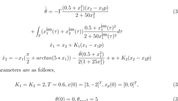
3.6 Simulation Examples
For illustration of the effectiveness of the proposed approach a simulation test has been
done on an modified example taken from [Primbs, 1999]. The purpose is to asymptotically
stabilize the Van der Pol system given by,
˙
x1 =x2 (28)
˙
x2 =−x1(
π
2 +arctan(5x1))−
5(0.5 +x21) 2(1 + 25x2
1)
+u (29)
where x1 and x2 are the states, uis the control input. The constructed ISS-CLF function is
Viss = 1 2x
2 1+
1
2(x1+x2)
2 (30)
We construct the minimization function,
J = Z t+T
t
(x21(t) +u2(t))dt (31)
s.t.
˙ x1 =x2
˙
x2 =−x1(
π
2 +arctan(5x1))−
5(0.5 +x2 1)
2(1 + 25x2 1)
+u
V(x(t+T))≤V(xiss(t+T)
T = 3, dt= 1, x0 = [3,−2]T
Results of the simulation is shown in the Figure 1. It is clear that the developed ISS-CLF
algorithm can stabilized the system easily.
In the next step we modify the system and consider stabilization of an amplifier with unknown
parameters. Consider the system defined by,
˙
Figure 1: (a) convergence of the system states to the origin
˙
x2 =−x1(
π
2 +arctan(5x1))−
θ(0.5 +x2 1)
2(1 + 25x2 1)
+u (33)
where x1 and x2 are the states, uis the control input, and θ is the unknown parameter. We
take the real value of θ = 5 and try to develop an estimation algorithm to converge to this
value.
J = Z t+T
t
(x21(t) +u2(t))dt (34)
s.t.
˙ x1 =x2
˙
x2 =−x1(
π
2 +arctan(5∗x1))− ¯
θ(0.5 +x21) 2(1 + 25x2
1)
+u
¯ θ= ˆθ
The estimation algorithm is as follows,
˙ˆ
θ =−Γ(0.5 +x
2
1)(x2−x2p)
2 + 50x2 1
(35)
+ Z
T
(xiss1 (τ) +xiss2 (τ))0.5 +x iss
1 (τ)2
2 + 50xiss1 (τ)2dτ
˙
x1 =x2+K1(x1 −x1p)
˙
x2 =−x1(
π
2 +arctan(5∗x1))− ¯
θ(0.5 +x2 1)
2(1 + 25x2 1)
+u+K2(x2−x2p)
where the parameters are as follows,
K1 =K2 = 2, T = 0.6, x(0) = [3,−2]T, xp(0) = [0,0]T, (36)
θ(0) = 0, θreal = 5 (37)
Results of the simulation shown in Figure 2 and Figure 3 prove the efficiency of the method
in estimation of the parameters of the system and also in optimal running of the system to
the origin.
Figure 3: the system state estimations and corresponding real values
3.7 Summary
In this chapter we introduced a method for adaptive receding horizon control of nonlinear
systems . Asymptotically stability and optimality of the closed loop systems in the presence
of parametric uncertainty has been shown based on input-to-state stabilizing Lyuapunov
control functions. At the end, we used two simulation to prove the efficiency of the proposed
Chapter 4
Passivity Based Parameter Estimation in Adaptive Control
of Nonlinear Systems
In this chapter a method for adaptive parameter estimation of nonlinear systems with
imperfect state measurement is introduced. Globally uniform boundedness of all system
signals in the presence of parametric uncertainty is obtained through stability analysis.
4.1 Introduction
There are control problems whereby the reference trajectory is not known a priori but
de-pends on the unknown parameters of the system dynamics. The controller finds the operating
set-points which optimizes a performance or cost function and tries to run the system to that
point. The uncertainty associated with the function makes it necessary to use some sort of
adaptation and perturbation to search for the optimal operating condition. However, the
main challenges with adaptive control approaches lies with the ability to recover the true
unknown values of the parameters. In most approaches exact reconstruction of the unknown
parameters in finite time (FT) is obtained provided a given persistence of excitation (PE)
condition is satisfied. A common approach to ensuring a PE condition in adaptive control is
to introduce a perturbation signal as the reference input or to add it to the target set point
or trajectory, however, this constant PE in many cases deteriorates the desired tracking or
regulation performance. Recently a finite time parameter estimation method is developed
in [Adetola and Guay, 2008] which introduces such a PE signal and remove it when the
parameters are assumed to have converged. In this chapter, we remove this assumption and
consider problems where only a part of the state and just the scalar plant output is available
for measurement. For these systems, we build exponentially convergent nonlinear observers
and replace the unmeasured states by their estimates. Then, develop a model predictive
control strategy to run the system to the origin and study stabilizing property of the
opti-mization problem in the next chapter.
concept of passivity has been used principally in network synthesis and became a fundamental
feedback control concept in Popov [Popov 1966].
Consider the system
˙
x=P(x, u) (1)
where x∈Rn is the state and u∈Rm is the input the system.
Definition 4.2.1:The System (1) is said to be passive if there exist a continuous nonnegative
storage function S : Rn ×R
+ → R+ which satisfies S(0, t) = 0,∀t ≥ 0 such that for all
u∈C0, x(0)∈Rn, t≥t
0 ≥0,
Z t
t0
yT(σ)u(σ)dσ≥S(x(t), t)−S(x(t0), t0). (2)
Definition 4.2.2: The System (7) is said to be strictly passive if there exist a continuous
nonnegative storage function S : Rn×R
+ → R+ which satisfies S(0, t) = 0,∀t ≥ 0 and a
positive definite function (dissipation rate) ψ : Rn → R
+, such that for all u ∈ C0, x(0) ∈
Rn, t≥t0 ≥0
Z t
t0
yT(σ)u(σ)dσ ≥S(x(t), t)−S(x(t0), t0) +
Z t
t0
ψ(x(σ))dσ. (3)
Lemma 4.2.1: Suppose the System (7) is strictly passive. If S is positive definite, radically
unbounded, and decresecent, then foru≡0 the equilibriumx= 0 of (7) is globally uniformly
asymptotically stable.
4.3 Problem Description
The considered system is the following nonlinear parametric affine system
˙
x=f(x, y) +F(x, u)Tθ, (4)
y=h(x, u), (5)
wherex∈Rnis the state,u∈Rmis the control input,y ∈Rris the output, andθ ∈Rp is the
unknown parameter vector to be identified which lies within an initially known compact set
in x as,
f(x, y) =
f1(x, y)
f2(x, y)
.. .
fn(x, y)
, F(x, y) =
F1(x, y)
F2(x, y)
.. .
Fn(x, y)
. (6)
Also f(0, t) = 0 and h(0, t) = 0 for all t≥0.
The main goal of this note is to provide the true estimates of the plant parameters in FT while
preserving the properties of the controlled closed-loop system and therefore it is assumed
that there is a known bounded control law to, upon the control objective, (robustly) stabilize
the plant and/or to force the output to track a reference signal.
To prepare for the parameter identification procedure to be presented in the next section,
we consider simplicity in the equation (5) as h(x, u) =eT1x and rewrite the system as,
˙
x=f(x, y) +F(x, u)Tθ, (7)
y=x1 =eT1x, (8)
however, emphasize that it implies no restriction on the whole parameter estimation
proce-dure.
4.4 Infinite Time Parameter Identification
Denoting the state predictor for (7) as ˆx we define
ˆ˙
x=f(x, y) +F(x, u)Tθˆ+A(x−xˆ), (9)
where ˆθ is a parameter estimate generated via the update law to be developed and the state
estimation error will be ε=x−xˆ with the dynamic governed by,
˙
ε=Aε. (10)
We introduce the filters
˙¯
Ω0 =−A( ¯Ω0+y)−f(x, y), (11)
˙¯
and denote the output estimation as,
ˆ
y = ¯Ω0+ ¯ΩTθˆ (13)
which result in output estimator error,
=y+ ¯Ω0−Ω¯Tθˆ (14)
Substituting (11) and (12) into (14) we get,
= ¯ΩTθ˜+ ˜ (15)
where ˜ is governed by,
˙˜
=−A˜+ε. (16)
We define the update law for ˜θ as,
˙ˆ
θ = Proj{Γ ¯ Ω
1 +ν|Ω¯|2}. (17)
Γ = ΓT ≥0, ν >0,
Lemma 4.4.1: Consider the operator D defined as,
D: ˜θ →Ω¯ (18)
˙¯
Ω = −AΩ +¯ F(x, u), (19)
= ¯ΩTθ˜+ ˜ (20)
˙˜
=−A˜+ε. (21)
˙ˆ
θ = Proj{Γ ¯ Ω
1 +νkΩ¯k2},Γ = Γ
T ≥
0, ν > 0 (22)
This system is strictly passive. Hence, the equilibrium = 0 and ˜θ = 0 are globally uniformly
stable.
Proof: Using (15) we will have,
Z t
0
( ¯Ω)Tθdτ˜ =
Z t
0
TΩ¯Tθdτ˜ =
Z t
0
=
Z t
0
(k− 1
2˜k − 1 4k˜k
2)dτ ≥ −1
4
Z t
0
k˜k2dτ
on the other hand from using (16) and (10) by letting c=λ(A) we have,
1 2
d dt(˜
2+1 ckεk
2
P)≤ −c˜
2+ε˜− 1
2ckεk
2 (24)
≤ −c
2˜
2− c
2(˜− 1
cε) 2
+ 1
2cε 2− 1
2ckεk 2
≤ −c
2˜
2 − 1
2ckεk 2.
Using this and (10) we can deduce,
d dt(
1 2kk˜
2)≤ −c
0k˜k2 (25)
with suitable choice of c0. Integrating this equation we come to,
−1
4
Z t
0
k˜k2dτ ≥ 1
2c0
k˜(t)k2− 1
2c0
k˜(0)k2+3 4
Z t
0
k˜k2dτ (26)
and substituting (26) in (23) we obtain,
Z t
0
( ¯Ω)Tθdτ˜ ≥ 1
2c0k˜(t)k 2− 1
2c0k˜(0)k 2+ 3
4
Z t
0
k˜k2dτ (27)
which proves that the operator (18) is strictly passive.
Remark 4.4.1: Using the globally uniformly stability of and ˜θ, based on the defined update
law we can show that θ˙ˆis bounded on its maximal interval of exitance.
Theorem 4.4.1: All the signals in the closed loop adaptive system consisting of the plant
(7)-(8), filters (11)-(12) and the update law (17) are globally uniformly bounded and in
particular, limt→∞= limt→∞θ˙ˆ= 0. and, limt→∞(ˆθ−θ) = 0.
Proof: Combining (11), (12) and (14), we get,
˙
=A0+F(x, u)Tθ˜−Ω¯Tθ˙ˆ (28)
Becuase of the boundness of all the signals, ˙ is bounded. Since is asymptotically stable,
hence,
limt→∞
Z t
0
˙
So, by Barbalat’s lemma we have ˙ → 0. Now, since, θ˙ˆ is globally uniformly stable, we
conclude that F(x, u)Tθ˜(t)→0, and if we provide the richness condition:
1
T
Z t+T
t
F(x, u)F(x, u)T ≥c0I, c0 >0 (29)
then, the parameter error ˜θ will converge to zero asymptotically.
Remark 4.2.2: The benefit of using this special formulation is that in construction of the
filters we dont need just to measure the whole state x.
Remark 4.4.3: The result in Theorem 4.4.1 is independent of the control input u.
4.4 Finite Time Parameter Identification
In this section we are going to formulate a finite time parameter identification algorithm.
Lemma 4.4.1: Consider again the equation (16) and(15),
= ¯ΩTθ˜+ ˜
˙˜
=−A˜+ε
Define,
µ=ε−θ˜ (30)
˙
µ=−Aµ, µ(0) =(0) (31)
and matrixes,
˙
Q=T, Q(0) = 0 (32)
˙
C =T(θˆ+ε−µ) (33)
Suppose there exists a time tc and a constant c1 >0 such that Q(tc) is invertible i.e.
Q(tc) =
Z t
t0
(τ)T(τ)dτ > c1I
Then,
θ =Q(t)−1C(t),∀t≥t0 (34)
Proof: consider,
Q(t)θ=
Z
Using the fact that −µ=θ˜, it follows that,
θ=Q(t)−1
Z
C(τ)dτ =Q(t)−1C(t).
Remark 4.4.1: The result obtained here is independent of the control u and parameter
identifier θ˙ˆ used for parameter estimation, Hence we use the nominal estimate θ0 with no
parameter adaption. So if
θc=Q(tc)−1C(tc)
The finite time identifier is,
ˆ
θc=
θ0 if t < t
c
θc if t > tc
The benefit of using this algorithm is that we can predict when PE condition of - invertibility
of Q - is satisfied and to turn off the identification machine after that.
4.6 Supporting Example
In this section we consider an example of identification in a nonlinear system to show the
efficiency of the proposed algorithm.
Consider the system,
˙
x21 =x2+x21θ (36)
˙
x2 =u (37)
with the parameters,
x0 = [0,10]T, θ0 = 0, θreal = 5
N = 8, dt= 0.1
The results of simulation show the efficiency of the proposed method. Figure 1 shows
conver-gence of the parameters estimation and the system input. It is clear that the system states
converges to the real values. Figure 2 shows the system state estimations and corresponding
real values. Estimation of the system state can track the real states of the system very well.
4.7 Summary
in-Figure 1: (a) shows convergence of the parameters estimation and (b) is the system input
uncertainty was obtained through stability analysis. In the next chapter results of this
chap-ter will be used to build up a model predictive control scheme to steer the system to the
Chapter 5
Adaptive Predictive Control of
Nonlinear Systems: An Application to a CSTR system
In this chapter a method for adaptive predictive control of nonlinear systems is presented.
This method is based on finite time identification algorithm derived in the last chapter. The
efficiency of the proposed scheme is examined on an example of the CSTR system.
5.1 Introduction
There are control problems whereby the reference trajectory is not known a priori but
de-pends on the unknown parameters of the system dynamics. The controller finds the operating
set-points that optimize a performance or cost function. The uncertainty associated with the
function makes it necessary to use some sort of adaptation and perturbation to search for the
optimal operating condition. One of the main challenges with model based or adaptive
con-trol approaches is the ability to recover the true unknown values of the parameters. In most
approaches exact reconstruction of the unknown parameters in finite time (FT) is obtained
provided a given persistence of excitation (PE) condition is satisfied. A common approach
to ensuring a PE condition in adaptive control is to introduce a perturbation signal as the
reference input or to add it to the target set point or trajectory, however, this constant PE
in many cases deteriorates the desired tracking or regulation performance. In last chapter
we introduced a finite time parameter estimation method which introduces such a PE signal
and remove it when the parameters are assumed to have converged.
In the present chapter , predictive control of uncertain nonlinear systems subject to state
and input constraint is considered. We develop a new adaptive predictive control scheme
that enjoy all the desired properties without becoming computationally prohibitive. The
scheme is based on two main ideas. First, by working on a suitable estimation scheme, it
is shown how to obtain a finite time estimation algorithm. Second, by use of the predictive
control strategy, the system is running to the desired stable point. Stability of the predictive
control algorithm is enforced by constraining the terminal state to belong to the estimated
5.2 Problem Statement
The system considered is the following nonlinear parameter affine system
˙
x=f(x, y) +F(x, u)Tθ, (1)
y=h(x, u), (2)
where x∈Rn is the state, u ∈Rm is the control input, y ∈Rr is the output, and θ ∈Rp is
the unknown parameter vector to be identified which lies within an initially known compact
set Ωθ. Also, it is supposed that f(x, y) and F(x, y) are smooth matrix valued function.
5.3 Parameter Identification Algorithm
In the last chapter a finite time identification algorithm has been developed that we review
here.
Denoting the state predictor for (1) as ˆx we define
ˆ˙
x=f(x, y) +F(x, u)Tθˆ+A(x−xˆ), (3)
where ˆθ is a parameter estimate generated via the update law to be developed and the state
estimation error will be ε=x−xˆ with the dynamic governed by,
˙
ε=Aε. (4)
We introduce the filters
˙¯
Ω0 =−A( ¯Ω0+y)−f(x, y), (5)
˙¯
Ω = −AΩ +¯ F(x, u), (6)
and denote the output estimation as,
ˆ
y = ¯Ω0+ ¯ΩTθˆ (7)
which result in output estimator error,
=y+ ¯Ω0−Ω¯Tθˆ (8)
Substituting (5) and (6) into (8) we get,
where ˜ is governed by,
˙˜
=−A˜+ε. (10)
Now consider
µ=ε−θ˜ (11)
˙
µ=−Aµ, µ(0) =(0) (12)
and matrixes,
˙
Q=T, Q(0) = 0 (13)
˙
C =T(θˆ+ε−µ) (14)
Suppose there exists a time tc and a constant c1 >0 such that Q(tc) is invertible i.e.
Q(tc) =
Z t
t0
(τ)T(τ)dτ > c1I
Then,
θ =Q(t)−1C(t),∀t≥t0 (15)
Remark 4.4.1: The result obtained here is independent of the control u and parameter
identifier θ˙ˆ used for parameter estimation, Hence we use the nominal estimate θ0 with no
parameter adaption. So if
θc=Q(tc)−1C(tc)
The finite time identifier is,
The benefit of using this algorithm is that we can predict when PE condition -
invert-ibility of Q - is satisfied and to turn off the identification machine after that.
5.4 Adaptive Predictive Control Scheme
The goal in this section is to design a MPC law to be implemented using the standard
nonlinear model predictive control techniques, with takes into account constraint imposed
on the process input, output and state variables.
The model predictive feedback is defined as,
u∗(·)≡argminu
[0,T]J(·), (17)
J(·) =
Z T
0
L(t,x, u¯ )dτ +W(¯x) (18)
˙¯
x=f(¯x, y) +F(¯x, y)θc, x¯(0) =x (19)
θc = ˆθ(τ) (20)
u(τ)∈U,x¯(τ)∈X, ∀τ ∈[0, T]
¯
x(T)∈Xf
5.4.1 Closed loop Robust Stability:
Robust stability is guaranteed if predicted state at terminal time belong to a robustly
in-variant set for all possible uncertainties. For computation of this inin-variant set, we let the
linearized dynamics of the system as
x(k+ 1) =A(θc)x(k) +B(θc)u(k), x(t) = ¯x, k ≥t. (21)
Under the assumption of the stabilizablity of the pair (A,B), we consider the control law,
u=KLQ(θc)x (22)
whereKLQ(θc) = (R+BT(θc)P B(θc))−1BT(θc)P A(θc) andP is the unique positive solution of the algebraic Reccati equation
P(θc) = AT(θc)P(θc)A(θc)+Q−AT(θc)P(θc)B(θc)(R+BT(θc)P(θc)B(θc))−1B(θc)TP(θc)A(θc). (23)
Hence, the linearized systemAcl(θc) :=A(θc)+B(θc)K(θc) is stable. We let a positive matrix
˜
Q, and γ be a real positive scalar such that γ ≤λminQ˜. Let Π(˜θ) be the unique symmetric
positive definite solution of the Lyapunov equation,
ATcl(θc)Π(˜θ)Acl(θc)−Π(˜θ) + ˜Q= 0. (24)
Then, there exist a constant c∈(0,∞) satisfying a neighborhood Xf(˜θ) of the origin of the
Criterion 5.4.1: For any, θ1 and θ2 ∈Θc, withkθ1k ≤ kθ2k, we have Xf(θ1)≤Xf(θ2).
Theorem 5.4.1: LetX0(Θ) denotes the set of initial states for which proposed MPC has a solution. Assuming criteria 1 is satisfied, then for the closed loop system state, x originating
from any x0 ∈X0 feasibly approaches the origin as t→ ∞.
Proof: Proof is very similar to the proof 4.2 in [Mayne and Michalska, 1990].
5.5 CSTR Dynamics
In this section, the new estimation and also adaptive MPC algorithm is applied to the
highly nonlinear model of a continuous stirred tank reactor (CSTR). Assuming the liquid
volume, the CSTR for an exothermic, irreversible reaction, A → B, is described by the
following dynamic model, based on a component balance for reactant balance for A and a
energy balance,
˙
CA=
q
V (Caf −CA)−k0exp(− E
RT)CA, (25)
˙
T = q
V (Tf −T) +
(−4H)
ρCp
k0exp(−
E
RT)CA+ U A V ρCp
(Tc−T) (26)
where CA is the concentration of A in the reactor, T is the reactor temperature, and Tc is
the temperature of the coolant stream. The constraints are 280K ≤ Tc ≤ 370K,280K ≤
T ≤ 370K,0 ≤ CA ≤ 1mol/I. The objective is to regulate CA and T by manipulating
Tc. The nominal operating conditions corresponding to the unstable equilibrium CAeq =
0.5mol/I, Teq= 350K, Teq
c = 300 are: q= 100I/min, Tf = 350K, V = 100I, ρ= 1000g/I, Cp =
0.239J/gK,4H =−5×10⁴J/mol, E/R= 8750K, k0 = 7.2×10¹⁰min−1, U A= 5×10⁴J/minK.
The nonlinear discrete time model of the system can be obtained by using the state vector
x = [CA−CAeq, T −Teq]T and the input u = Tc−Tceq and discretzing with the sampling
time 4t= 0.01min. Let Q= diag(1/0.5,1/350), and R = 1/300, and ˜Q= 0.05I, λ = 0.01,
yielding c= 0.0915.
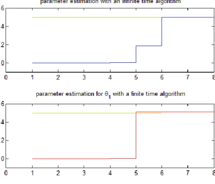
In the simulation, we have consideredθ1 :=k0 andθ1 :=k04Has uncertain parameters with
the starting valuesθ1(0) = 6×10¹⁰, θ2(0) = 5×6×1014. Convergence of the parameters with
estimation machine after a definite time. Using the finite time algorithm we have controlled
the SCTR system employing the proposed adaptive predictive scheme. Results, shown in
figure (3) indicates the convergence of the parameters to the origin.
Figure 1: convergence of the parameters estimation in (a) infinite time algorithm (b) finite
time algorithm
5.6 Summary
In this chapter a method for adaptive predictive control of nonlinear systems was presented.
This method is based on finite time identification algorithm derived in the last chapter. The
Figure 2: convergence in the parameters estimations for θ0 = [4×1010,5×9×1017]
Figure 4: convergence in the state estimations for θ0 = [−4×1010,5×9×1017]

![Figure 2: convergence in the parameters estimations for θ 0 = [4 × 10 10 , 5 × 9 × 10 17 ]](https://thumb-us.123doks.com/thumbv2/123dok_es/5986489.167970/46.918.216.636.196.572/figure-convergence-parameters-estimations-θ.webp)
![Figure 4: convergence in the state estimations for θ 0 = [−4 × 10 10 , 5 × 9 × 10 17 ]](https://thumb-us.123doks.com/thumbv2/123dok_es/5986489.167970/47.918.215.634.197.569/figure-convergence-state-estimations-θ.webp)
