A parametric study trying to optimize the performance of the code was performed on the following variables: ILU fill levels, inexact-Newton convergence parameter, residual reduction tolerance parameter to switch to the inexact Newton phase, and a preconditioning parameter used in the formation of the approximate Jacobian. 49 6.1 Comparison of TYPHOON surface velocity profile against Blasius solution 52 6.2 The computational grid used in the Blasius solution comparison.
Motivation
Background
Unstructured grids are typically used in combination with finite volume schemes, while structured grids can be solved with both finite volume and finite difference schemes. Unstructured grids can be generated on much more complex geometries and refinement on a particular region in the flow field can be achieved by splitting cells as needed.
Objectives
The focus of this thesis is to apply the full Navier-Stokes equations to the existing algorithm and to integrate the Spalart-Allmaras turbulence model into the flow equations. Governing equations, where ρ is the density, ρu, ρv, and ρw are the components of momentum, and e is the total energy.
Turbulence Model
Curvilinear Coordinate Transformation
Boundary Conditions
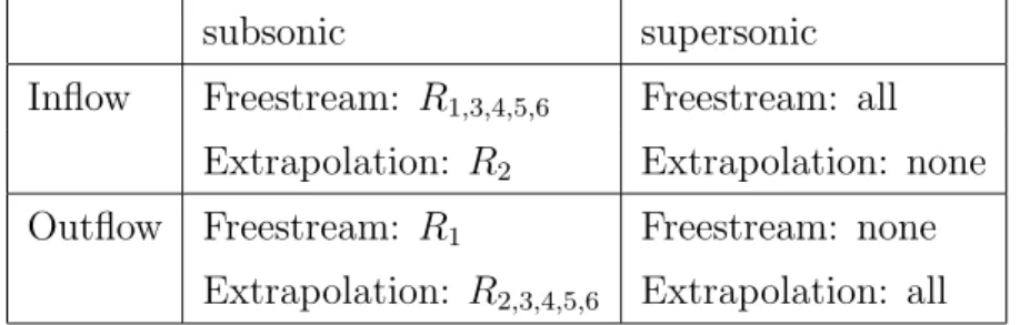
- Far-field Boundary
- Solid Wall
- Inviscid Fluxes
- Viscous Fluxes
- Turbulence Model
- Boundary Conditions
Thus, the following compact three-point template (developed by Pulliam in [29]) is used:. are the α values at the half-points of the nodes in the ξ direction. As discussed in Section 2.4.1, the choice of inviscid far-field boundary conditions depends on the inflow or outflow conditions at that point.
Linearization and Newton’s Method
Linearization of the Interior Scheme
Note that the entries a16 to a56 are zero, while the off-diagonal terms a61 to a65 originate from the vortex terms in the Spalart-Allmaras equation. The differentiation of the turbulence model can be done without much difficulty, since all terms correspond to the model in two dimensions.
Linearization of the Boundary Conditions
The turbulence model is included in the flow Jacobian in the following way: where the entries in the 5×5 block in the upper left corner of the matrix correspond to contributions from the Navier-Stokes equations, and the sixth row and column are from the turbulence model. The differentiation of the vorticity term can be found in Appendix B. Numerical Algorithm Newton's method as applied to this set of equations yields:. The selection of the flow variables in R necessitates a transformation of the update ∆R back to the workflow variables ˆQ.
Linearization of the viscous outflow far-field boundaries can be represented in the same general form as that of the viscous solid boundary in Equation 3.69, where instead, the Jacobians are:
Solution to the Linear Problem
- Jacobian-free GMRES
- Inexact-Newton Method
- Preconditioner
- Incomplete LU Factorization
- Reverse Cuthill-McKee Nodal Reordering
The flux matrix can become numerically stiff when a large spread in the eigenvalues is encountered. This reduces the efficiency of the GMRES solver as the equations become more difficult to solve. The preconditioning matrix can be applied to the left or right of the flow matrix, but right preconditioning is chosen since the residual is left unchanged.
The preconditioner is formed using an incomplete lower-upper factorization based on the approximate Jacobian of the current A1. The filling factor k allows the user to choose the precision of the matrix M with respect to the approximate Jacobian of the flow. A natural ordering of the terms in the Jacobian of the current produces a sparse matrix with high bandwidth.
The objective of the Reverse Cuthill-McKee method [5] is to rearrange the equations in such a way that the matrix entries are clustered near the diagonal, resulting in a reduction in bandwidth. This is important to reduce the storage requirements and improve the performance of the ILU factorization algorithm [27].
Algorithm Startup
Local Time-Stepping
The pseudo-time term for the mean flow equations during the approximately Newtonian phase is determined locally according to the work done by Pulliam in [29] and is given by: . 3.80), where Jj,k,m is the local Jacobian metric and ∆tref is the global reference time step, which increases as the solution evolves. Once an intermediate flow solution is obtained, the imprecise Newton method without the Jacobian is used. This clipping method was discovered by Chisholm [3] and Wong [37] to improve the stability of the solver.
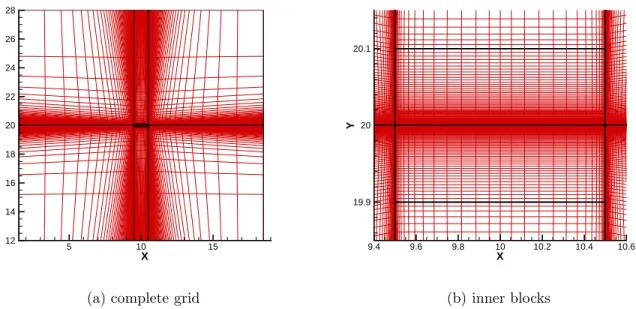
The manner in which the meshes are generated plays a critical role in the convergence of the flow solution.
Problem Definition
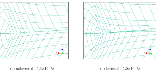
The algorithm for computing the determinant in ICEM involves computing all 27 metric Jacobians in a 27-node hexahedron at each cell volume. Thus, ICEM may report negative determinants indicating inverted cells when the grid is actually usable. The reverse can also happen, where non-negative determinants appear as inverted nodes in TYPHOON.
Smoothing
This method is generally desirable since the spatial discretization is most accurate on orthogonal grids, and the transformation of the equations into curvilinear coordinates produces the fewest terms [6]. The stabilization factor should be chosen as low as possible to improve the orthogonality of the joints outside the wall. The number of iterations should also be minimized as the algorithm will inevitably try to refine the mesh near the wall surface at the expense of the viscous space outside the wall.
In addition, the wing faces must be raised and the "define edges" option must be selected so that the distribution of nodes at the wing edges is also prevented from changing. A word of caution to begin this chapter: convergence rates were found to be quite network dependent. The parameters that are optimized in this section were found to be optimal for the networks that the author was able to generate.
The parameters here are optimized under the assumption that each is independent of the others. A multiblock configuration of twelve blocks around an ONERA M6 wing is used with the parameters prescribed in Table 5.2.

Parametric Study
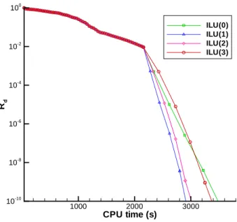
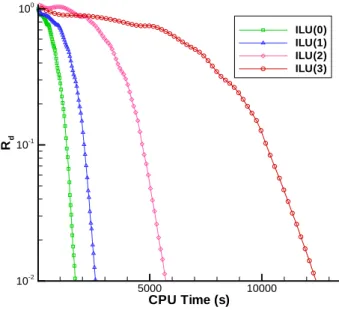
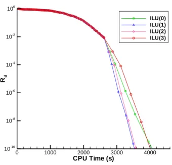
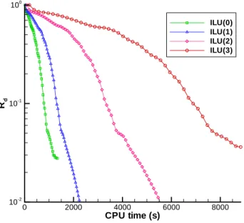
- ILU Fill Level (k)
- Preconditioning Parameter (σ)
- Inexact-Newton Parameter (η)
- Approximate-Newton Convergence Parameter (R d tol )
The preconditioning parameter σ combines the second and fourth difference dissipation terms in the preconditioner, as discussed in Section 3.2. In the laminar regime, it was found to be optimal at values of 4.0 for transonic flow, and 6.0 for subsonic flow (see Figures 5.9 and 5.10). Note that the flow solver had difficulty converging the flow for values below six in the approximate Newtonian phase of the subsonic flow solutions.
The best turbidity values were found to be 3.0 for subsonic and transonic flows (see Figures 5.11 and 5.12). For laminar flows, the parameter was found to be strongest for values of approximately 0.1 during the approximate Newtonian onset phase. Turbulent flows required values of 0.1 for both Newtonian and Jacobian-free phases.
This threshold parameter controls the transition from the approximate Newton boot method to the Jacobian-free method. A well-chosen reduction parameter will reduce the amount of time the algorithm takes to converge, while preventing divergence in the solution.
Summary of Optimal Parameters
Blasius Solution
The Blasius equation is an exact solution of the boundary layer equations for a steady incompressible two-dimensional flow over a flat plate at a zero degree angle of attack. It was shown by Blasius that under these conditions the boundary layer equations can be reformulated into a single third-order ordinary differential equation simply by choosing an appropriate coordinate transformation. The velocity profile obtained from TYPHOON is compared with the velocity profile obtained from the solution to the Blasius equation.
TYPHOON shows the basic shape closely with slight overshoot, but at most, the error between the Blasius solution and TYPHOON is about 2%.
NACA0012 Airfoil
The results for the laminar cases are shown in Figures 6.3 and 6.4, while the results for the turbulent cases are shown in Figures 6.5 and 6.6. The correlation between the two codes is quite good for all cases with small discrepancies in the transonic turbulent case likely attributed to the use of the full Navier–Stokes equations in TYPHOON as opposed to the thin-layer Navier–Stokes equations in OPTIMA-MB. The CPU temporal unit of measure is the equivalent evaluation on the right-hand side defined as the total CPU time divided by the time for one evaluation on the right-hand side.
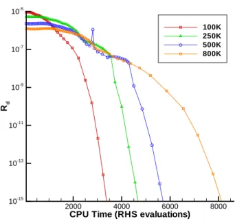
Grid Convergence Studies
A summary of the grid characteristics is shown in Table 6.4 and flow results at six spanwise locations are shown in Figure 6.9. Convergence histories for the three grids are plotted as a function of equivalent right-hand evaluations in Figure 6.10. The results show that the grids used tended to cause TYPHOON to underpredict the pressure coefficient at the leading edge, while overpredicting it at the trailing edge.
Increasing the grid points in the flow field appeared to improve the solution somewhat, but the inability to finer the spacing at the leading edge and wingtip prevented further studies of the effects of a finer grid. To improve the efficiency of the solver, the linear system is preconditioned using an incomplete lower/upper factorization of the approximate Jacobi matrix and solved imprecisely. A first-order approximation to the Jacobian is used in the initial stage of running the convergence of the solution, and later it is switched to a faster Jacobian-free method.
A numerical study has been carried out to optimize the parameters for the viscous and turbulent terms in the code. A mesh convergence study was also performed for an ONERA M6 airfoil at subsonic flow conditions for both laminar and transonic cases.
Recommendations
Chisholm, A Fully Coupled Newton-Krylov Solver with a One-Equation Turbulence Model, PhD-afhandling, University of Toronto, 2007. Zingg, A Fully Coupled Newton-Krylov Solver for Turbulent Aerodynamic Flows, Paper 333, ICAS 2002 Kongressen, sept. Godin, Turbulence Modeling for High-Lift Multi-Element Airfoil Configurations, PhD-afhandling, University of Toronto, 2004.
Leung, Parallel implementation of a Newton-Krylov flow solver on unstructured grids, Masters thesis, University of Toronto, 2004. Zingg, A Newton-Krylov algorithm for aerodynamic design using the Navier-Stokes equations, AIAA Journal pp. Nichols, A Three-Dimensional Multi-Block Newton-Krylov Flow Solver for the Euler Equations, MASc thesis, University of Toronto, 2004.
Zingg A Three-Dimensional Multi-Block Newton-Krylov Flow Solver for the Euler Equations, AIAA Paper. Pueyo, An efficient Newton-Krylov method for the Euler and Navier-Stokes equations, PhD thesis, University of Toronto, 1998. Zingg, Three-Dimensional Aerodynamic Computations on Unstructured Grids Using a Newton-Krylov Approach, AIAA Paper Toronto, ON June 2005.
Wong, A Compressible Navier-Stokes Flow Solver Using the Newton-Krylov Method on Unstructured Grids, PhD thesis, University of Toronto, 2006.
Logic for far-field boundary conditions using Riemann invariants
Orthogonal smoothing parameters in ICEMCFD
ONERA M6 wing test cases
Grids used in the ONERA M6 wing parametric study
List of parameters in the numerical study
Summary of results from parametric study
Flow conditions for the 2D validation test cases
Summary of grid characteristics used in the 3D laminar convergence study 58